A Quick Method for Judging the Feasibility of Security Constrained Unit Commitment Problems within Lagrangian Relaxation Framework

A Quick Method for Judging the Feasibility of

Security-Constrained Unit Commitment Problems within

Lagrangian Relaxation Framework

*

Sangang Guo

School of Mathematics and Computer Science, Shaanxi University of Technology, Hanzhong, China Email: [email protected]

Received September 7, 2012; revised October 10, 2012; accepted October 22,2012

ABSTRACT

Generally, the procedure for Solving Security constrained unit commitment (SCUC) problems within Lagrangian Re-laxation framework is partitioned into two stages: one is to obtain feasible SCUC states; the other is to solve the eco-nomic dispatch of generation power among all the generating units. The core of the two stages is how to determine the feasibility of SCUC states. The existence of ramp rate constraints and security constraints increases the difficulty of obtaining an analytical necessary and sufficient condition for determining the quasi-feasibility of SCUC states at each scheduling time. However, a necessary and sufficient numerical condition is proposed and proven rigorously based on Benders Decomposition Theorem. Testing numerical example shows the effectiveness and efficiency of the condition. Keywords: Security Constrained Unit Commitment (SCUC); Lagrangian Relaxation; Benders Decomposition

Feasibility Theorem; Ramp Rate Constraint

1. Introduction

Security-constrained Unit commitment (SCUC) is one of the most important daily functions for independent sys-tem operators (ISOs) to clear the electric power market and for generation companies (GENCOs) to analyze ge- neration costs and determine bidding strategies [1-3]. The objective of SCUC is to minimize the total bid cost in current electric power market or generating cost in traditional power systems while satisfying the system constraints including system demand balance, system spinning reserve and related transmission security con-straints, and individual unit operating limits such as minimum/maximum generation level, minimum up/down times, ramping rate constraints.

Since the SCUC is an NP-hard mixed integer-pro- gramming problem, it is extremely difficult to obtain the exact optimal solution within acceptable time [4]. La-grangian Relaxation (LR) is one of the most successful methods for obtaining suboptimal solutions [5], where Lagrange multipliers relax the system-wide constraints such as system demand balance, system spinning reserve and DC transmission constraints. Some methods, usually heuristics are needed to modify the dual solution into a feasible one. In fact, the Lagrangian based SCUC methods

are all similar but the ways to obtain feasible solutions may vary significantly.

It is clear that the core to develop an effective method for solving SCUC problems within the Lagrangian re-laxation framework is how to obtain feasible solutions. First of all, a necessary or sufficient condition used for checking promptly on the feasibility of SCUC states is crucial. Our previous work [6] proposed such conditions. However, a necessary and sufficient condition for deter-mining the feasibility of SCUC states at each scheduling time is not given. Furthermore, ramp rate constraints are not taken into consideration in those results.

A necessary and sufficient condition for determining the feasibility of SCUC states at each scheduling time is proposed and proven rigorously in this paper based on the Benders Decomposition Feasibility Theorem [7,8]. The condition is very crucial for constructing a feasible solution of a SCUC problem. Numerical test example shows that the presented condition is very efficient.

2. Problem Formulation of SCUC Problems

For the convenience of presentation, some notations are defined as follows.

T : commitment horizon in hours;

*_{The research presented in this paper is supported by the Natural}

Sci-ence Foundation of the Education Department of Shaanxi Province (11JK0498).

I: number of units with the index denoting the

unit;

i

th

 

i

P t

 

u t ith

t

 

 



: power generation by unit i at time t;

i : binary variable: 1 if the unit is turned on or kept on during the time period , else 0;

i

x t i

 

x t

: the number of time periods that Unit has been up ( _i 1)or down (x t_i

 

 1);

i

 : the minimum number of time periods for which the unit must be up; i

i: the minimum number of time periods for which

the unit must be down; τ i

 





C P ti i : fuel cost of producing power P ti

 

i

   



,



i i

S x t u t i

 

D t t

 

P t t

for thermal unit ;

i

: total demand of the whole power system during time period ;

: startup/shutdown cost for unit ;

r : the spinning reserve requirement during time period ;

 

i

r t :

 



r P, P t

 



t

min

r ti  i i i is the spinning

re-serve requirement during time period , r_iis the

maxi-mum spinning reserve requirement;

it: the maximum generation of unit at scheduling

time , if unit has no raping limit, P t i PitiPi;

it: the minimum generation of unit at scheduling

time , if unit has no raping limit, P t i PitiPi 







,u ti 1



 _{   }

 _{ }

 

 

 

i u ti D t

 

D t k

 

 

i u ti P tr

;

i

The objective of the unit commitment problem is to minimize the total operating cost as the following mixed integer-programming problem:

: the maximum ramp rate;

 





 

 

1 1

min T I i i i i i

t i

C P t u t S x t

 



, (1)

subject to

2.1. System Level Constraints

1) System demand constraint

 

1

I

i

P t





, (2) where k is the demand at bus ;

2) Spinning reserve constraint:

 

1

I

i

r t





, (3)

where r ti

 

min



r Pi, iP ti

 



is the maximum

spin-ning reserve requirement.

3) Transmission security constraints:

 

,

 

 

1 1

1, , ,

I K

l l l i i

i k

, ,

l k k l

F F t P t

l L

 

     









D t F

  ₍₄₎

2.2. Individual Unit Constraints

4) The minimum up/down time constraint:

 

, if



1



i i i

x t  u t 1,u t_i

 

0, (5)



 

, if 1 0, 1

i i i i

x t  u t  u t 

 

, (6) 5) The relation between the unit state and unit up/ down decision











 



 



  

1 1 ,if 1 1 1 ,if 1 1

i i i i

i

i i i

x t u t x t u t

x t

u t x t u t

      

  

   

 (7)

6) Generation constraint

 

 

 

 

,if 0, 0, if 0.

it i it i

i i

P P t P x t

P t x t

   

 

 

 (8)

7) Ramp rate constraints: if



1



1 and

 

1

i i

x t  x t  then

 



1



i i i

P t P t   , (9)

8) Minimal power generation constraint at the first/last up hour:

 



   







,

 

, 0,

ifi i 1i i ii 1i

P t P r x t P t

u t u t

 

  

 

 

, min, , 0 , y Y z Z g y z

(10)

3. The New Necessary and Sufficient

Condition for Checking the Feasibility of

SCUC States

A mixed-integer programming problem can be repre-sented as

f y z

  

n

YR

, (11) where is assumed to be a nonempty convex set and g is concave on Y for each fixed m,

z Z R

y

and are continuous and discrete variables, respec-tively.

z

z Z

0

y Y

Definition: A vector ₀ is called to be quasi- feasible if there exists a vector such that



,



0

g y z 

Y

0 0

Benders Decomposition Feasibility Theorem [7,8]: For problem (11), and

.

Z are nonempty and is

convex, the vector function

Y

 

,

g y z

z Z

is concave vector function for each  . Furthermore, the set



m|

 

, for some



z

W  wR G y z w yY

z Z

(12) is closed for each  . Then 0 is quasi- feasible if and only if the following inequalities are satis- fied for

z ZV

   

 

sup



, 0



0

T

y Y

c   g y z

 , (13)

 

1

| 0, m i 1

i

  

 where

 

    





, (14)



:

 

, 0,for some





Note 1: The result still holds for all  0

Note 2: A SCUC problem can be written as the form of

. Equation (11), where



i1, , in



, ,

y y y Y P P_{1 1} P P 

n n

i t i t i t i t

 

   

 

 

 

scartes product 24 0,1

1 0,1

   , (17) and n is the number of generating

time t, i are the indices of generating units,

      , (16)

De

0,

Z



units at scheduling

k Pit and

it

P a the minimal and maximal power generation of unit i lev l, pectively.

 

,

re

e res g y z is a 2L3-dime onal

ctor function, of which the first and second dimensions orresponds to the syste and co

constraint can be represented as two inequalities), the third relates to the spinning reserve constraint, and the rest dimensions correspond to 2L transmission security

constraints.

 

,

nsi ve

c m dem nstraint (since such

f y z is the total cost including the fuel

cost of all generating units at e t and their startup

cost.

Since for SCUC state vector zZ at each

schedul-ing tim

tim

e t the neration of units not being

st the se

power ge

arted up need not be optimized, t Yis determined

by z and is a convex cube of Rn. For the given SCUC

state vector zZ, g y z

 

, is the cont uous concave

vect function over the closed c vex set Y, and hence

in on or

z

W is closed ach scheduling time t, the

SCUC problem is a mixed-integer programming of the (11), which satisfies the conditions of the above Benders Decomposition Feasibility Theorem.

To obtain the desired result, the units are classified into three categories at time t: E is the set

. Th form of units w ho E

, E

erefore, at e

1t

hich is on the normal generating state; E_2t is the set

of units at the first/last generating ur; E3t is the set of

units with ramp rate constraints. The set 3t is further

classified into four types, named as 0 3t

E ₃1_t, E₃2_t and

3 3t

E respectively, as follows:

 

 

 

















0

3t | 3t, i 1, i 1 st t 1

E  i iE x t  x t   i

1 3 3 2 3 3 3 3 3 ,fir las | , | , | ,

t t it i i

it

t t i i

it

t t i i it

E i i E P P r

E i i E P r P

E i i E P P r P

 

   

   

    

Using the Benders Decomposition Feasibility Theorem, we obtain the desired necessary and sufficient condition fo

value of the following no

r SCUC states to be feasible.

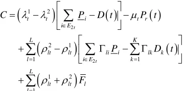
Theorem: SCUC states at scheduling time t is quasi-

feasible if and only if the optimal nlinear program is nonnegative:

 

minc

  , (18)

where

 



















1 1 0

1 3 3

1 3 1 3 2 3 3 2 3 3 3 , 0 3 ,0 , 3 , 0 3 , 0 3 3 , 3 3 , t i

t i t

t i t

t i t i t i t i i i i E

i i i i

i E

i

i i i

i E i E

it

i i

i E

i it i i E

it

i i

i E

i it i

i E

c P r

P r P P P r P r P P P P                                                   _   _        _  _    _   _    _   _



i





























  

 





 





3 3 3 3 3 3 3 3 2 3 , 0 3 ,0 3 3 ,

1 2 3

3 3 1 1 3 3 1 t i t i t i t it i i i E

i i i i

i E

i it i

i E

i

i r

i E

L K

L l l lk k

l k

L

l L l l l

P r

P r

P P

P D t P t

D t F                                            _   _    _   _         















and





1 2

1 2 3

1 2

3 3

1 2 2 1

1

, ,

, , 1, ,

t t t

l lt L l lt

L

i t t lt lt li

l l L                            



  

Proof: The left hand side of the Benders ecomposi-tion Feasibility Theorem is

D





 

 

 

 

 

 





 

 

 

2 3 1 3 1 2 3 2 1 1 1 m t t t t t t t

i E i E

t i i r

i E i E

L

i

lt lt li i li

l i E i E

K

li i lk k

i E k

1

1 2

ax

t

i

t t i i

i E

P t P P t D t

 



r t r t P t

P t P

P t D t

                _{   }           _   _       _  _          

















 







   





       1 2 1

, , min ,

max ,

t it i it i i i i

L

lt lt l

l

i i i

i E P P t P r t r P P t

F

f P t r t C





 





 

 





2 2 1 2 2 1 1 2 1 t t i t t i E i

lt lt li

l i E

L

lt lt l

l C P F               _  _       









1 1 t r L K lk k k

D t P t

P D t

         





The solution of problem (19) depends on the following subproblems since the problem (19) is decomposable with respect to units:

i) Subproblem 1: iE1t, we have

        





 

 



 

 



 

 











 

 



 

 

, min ,

3 * * * * 3 max ,if 0, ,if 0 ,

,if , ,

i i i i i i i

i i P P t P r t r t P P t

i i

i i i i

i i i i i

i i i i i

i i i i i

f P t

P t

P r P t

P r

P t P r r t r

P P t P

                 _{ }   _{   }            * * 3 3 , , , 0 i t i

i i i i

r t

r t

P r t r

r t

 



 



ii) Subproblem 2:

i



E

₃0_t, we have

      



   



      

 

 

 

 

3 in ,

,if , 0

i

i i i

r

i i

iP P ti P ri t



  

3:

i



E

1_3t, we have , min ,

, m

max ,

max

it i it i i it i

i i i

P P t P r t r P P t

P P t P r t

f P t r t

P t r t

 

   

  

 

* *

it i it i PitP ti

iii) Subproblem

      



   



      

 

 

 

 

 

 

, min ,

, min ,

3 3 max , max ,if 0, ,if 0,

it i it i i it i it i it i i it i

i i

P P t P r t r P P t

i i

P P t P r t r P P t

it

i i i i

i it i i i

f P t

P t

P r P t

P r P t

                       3 * * * * , , i i

it i i

it i i

r t

r t

P r t r

P r t r

 

 

 

 

iv) Su m 4: 2 3t

iE , we have

bproble       



   



      

 

 







 

 









 

 



in , 3 , min ,

3 3 * * 3 3 * * , max ,if , , , ,

it i it i i it i

it i it i i it i

i

r P P

i i i

P P t P r t r P P t

it it

i i i

it

i it i it i

i it i i it

r t

,maxm i i

P P t P r t t f P t

,if

it

i i i

P t r t

P P P

P t P r t P P

P

P t P r t P P

              _{  }   _{  }      

v) blem 5: 3 3t

iE , we have

P P               Subpro       





  



      

 

 

 

 











 

 









 

, min ,

3 , min ,

* * 3 3 3 * * 3 3 * * max , max

,if 0, ,

,if ,

,

,if ,

,

it i it i i it i

it i it i i it i

i i i

P P t P r t r P P t

i i i

P P t P r t r P P t

it it

i i i i i i

i

i i i i i

i it i it i

i it i

f P t r t

P t r t

P r P t P r t r

r

P t P r r t r

P P P

P t P r

                    0

i Pi r _i i

              

 

   



i it

t P P

          

By Benders Decomposition Feasibility Theorem, we have the desired result. Q.E.D.

Note 3: The all subproblems above are linear pro-gramming problems with simple constraints. Thus, by comparing the values of all extreme points, the optimal solutions and corresponding optimal values can be ob-ta

Note 4: It should be noted that the theorem still hold for 0

 

ined easily.

  .

4. The Numerical Solution of the Problem

Consider the SCUC problem at scheduling time t with

0 being the objective



0



max 0, , 0,

,

g y z

y Y   _     (20)

where y, Yand Z are defined in Equations (16)-(17).

The dual problem of the problem (20) is

 

0

minc

  , (21)

By the theorem and the note 4, z₀ is quasi-feasible if

and only if and only if the optimal value of c

 

 is

nonnegative over the positive orthant  0. While the problem (21) can be solved by using subgradient method [9], and the value c

 

 can be obtained by Equation

(19) for the given Lagrange multiplier vector , the Lagrange multiplier can then be updated by subgradient method. S ce the best multiplier vector in the dual itera-in

lier tion of the SCUC problem is taken as the initial multip

0

 , the rate of convergence of  is quite promptly.

5. Numerical Testing Result

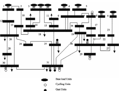
The standard IEEE example [5] tests the effectiveness and efficiency of the proposed me

has 16 units, 43 transmission lines,

is load bus). The fuel cost function of unit i is

[image:4.595.83.265.87.177.2]

 





2

 

 

i i i i i i

C P t a P t b P t Table 1. Generation level and its coefficient of fuel cost

function of each unit.

The data of units, the system reserve requirementP tr

 

, scheduling time

t

, the the system demandD t

 

at each

maximal value of DC power flow Flon each

transmis-sion line l and the amount of electric power on each

load bus are given in Tables 1-5, respectively. Units 1 and 4 have minimal power generation constraint at the first/last up hour.

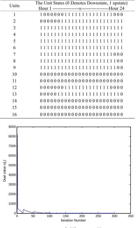
The CPU-time is within 2.3 second for checking SCUC states for 24 scheduling period on a DELL Computer with 2G RAM using MATLAB 7.01. Table 6 gives a feasible SCUC obtained within Lagrangian framework. Figure 2 presented the tendency of c

 

 k with  k

8

t . Testing example shows that the num

at erical

SCUC is

ef-T istence of ramp rate constraints and transmission con-straints increases the difficulty of obtaining an analytical co

ng o

d method for determining the feasibility of a fective and efficient.

6. Conclusions

The key of solving SCUC problems is to determine whether a SCUC is quasi-feasible or not. he ex

security ndition. However, a numerical necessary and sufficient condition for checki n the feasibility of SCUC states at each scheduling time is propose and proved rigo- rously based on Benders Decomposition Feasibility

Unit i Pi (MW)

i

P

(MW) i

r

(MW)

ai

(k$/MW2) (k$/MW)bi

1 300 1350 1000 0.0015 8.752

2 360 1620 1200 0.0016 7.654

3 360 1620 1200 0.0016 7.654

4 360 1620 1200 0.0016 7.654

5 300 1875 1500 0.0013 6.052

6 300 1875 1500 0.0013 6.052

7 240 1080 800 0.0015 9.072

8 150 675 500 0.0015 8.752

9 100 625 500 0.0015 8.752

10 45 202.5 150 0.0019 12.54

11 90 405 300 0.0018 11.62

12 120 750 600 0.0017 9.543

13 150 937.5 750 0.0015 8.352

14 52 235.7 175 0.0019 13.00

15 60 270 200 0.0018 14.62

16 120 750 600 0.0017 9.543

[image:5.595.102.494.417.717.2]

16

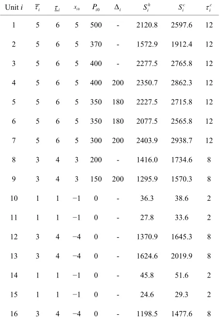
Table 2. Length of up/down time, initial states and coeffi-cient of startup cost function of each unit.

[image:6.595.59.286.114.447.2]

Unit

Table 4. Limits of DC power flow Fl on each transmission line.

Line: i > j Capacity_(MW) Reactance _(p.u.) Line: i > j

Capacity (MW)

Reactance (p.u.)

0

i

P i

i i i 

h i

S c

i

S c

i 0

i

x 

1 5 6 5 500 - 2120.8 2597.6 12

1 - 2 1000 0.025 16 - 18 1200 0.01

2 5 6 5 370 - 1572.9 1912.4 12

3 5 6 5 400 - 2277.5 2765.8 12

4 5 6 5 400 200 2350.7 2862.3 12

5 5 6 5 350 180 2227.5 2715.8 12

6 5 6 5 350 180 2077.5 2565.8 12

7 5 6 5 300 200 2403.9 2938.7 12

8 3 4 3 200 - 1416.0 1734.6 8

9 3 4 3 150 200 1295.9 1570.3 8

10 1 1 −1 0 - 36.3 38.6 2

11 1 1 −1 0 - 27.8 33.6 2

12 3 4 −4 0 - 1370.9 1645.3 8

13 3 4 −4 0 - 1624.6 2019.9 8

29.3 2

3 4 −4 0 - 1198. 1477 8

1 - 12 1000 0.008 16 - 19 800 0.01

2 - 13 1000 0.054 17 - 21 1200 0.015 3 - 14 2000 0.01 18 - 25 2500 0.0005

3 - 15 2000 0.01

19 - 26 (Double

lines)

250 0.045

4 - 6 1500 0.01 19 - 31 200 0.04

5 - 6 1500 0.01 20 - 24 1000 0.03

6 - 7 1200 0.015 20 - 28 1000 0.025 6 - 18

(Double lines)

1200 0.046 20 - 30 1000 0.05

7 - 16 1200 0.025 21 - 26 900 0.01

7 - 17 1200 0.015 22 - 26 1250 0.01 23 - 27 1250 0.01

3 1000 0. 2 1000 0.01

1 1000 0.0035 ou

lines)

045

12 - 20

(D 1000 0.05 800 0.01

13 - 1000 26

-13 - 1000 28

14 15

-14 1 1 −1 0 - 45.8 51.6 2

15 1 1 −1 0 - 24.6

[image:6.595.304.534.118.582.2]

16 5 .6

Table 3. System load and system reserve requirement for 24 sch lin ou

Hour

edu g h rs.

t D t  (M ) W

 

r

P t _Hour 

(MW) t



D t

W (M )

 

r W

P t

(M )

1 2502 250.2 13 7995 799.5

2 2441 244.

3 2197 219.7 15 6591 659.1

4 2075 207.5 16 6225 622.5

5 2502 250.2 17 6652 665.2

6 3418 341. 2

80 19

85 20

95 21 88 18.

7 76 22 28 02.

8 05 23

12 8300 830 24 2807 280.7

1 14 7201 720.1

8 18 7812 781.

7 4809 4 .9 8056 805.6

8 5859 5 .9 7079 707.9

9 6957 6 .7 51 5 8

10 690 9 40 4 8

11 056 8 .6 3174 317.4

8 - 22 1000 0.01

9 - 2 01 24 - 5 2

0 - 14 (D25

-31

ble 250 0.

11 - 15 1000 0.0035 26 - 27 1200 0.025

ouble lines)

4 26 - 29

18 0.03 31 600 0.0333

20 0.01 30 1000 0.025

18 1780 0.00815 30 - 31 700 0.022 18 1780 0.00815

le 5. nt o lo aw ad

us Per us Pe

Tab Perce f system ad dr n by lo bus.

B cent B rcent

1 0.024 7 0.265 2 0.024 8 0.062 3 0.361 9 0.024

4 0.0 0.

0

[image:6.595.58.284.487.737.2]

[image:7.595.56.291.112.502.2]

Table 6. A Feasible SCUC obtaine within Lagrangian re-laxati

d on framework.

Units The Unit States (0 Denotes Downstate, 1 upstate) _{Hou 1 --- ---s--- ---Hour 24 r --} --1 1 0 0 0 0 0 0 1 1 1 1 1 1 1 1 1 1 1 1 1 1 0 0 0 2

3

0

1 1 1 1 1 1 1 1 1 1 1 1 1 1 1 1 1 1 1 1 1 1 1 1

0 0 0 1 1 1 1 1

1 1 1 1 1 1 1 1

5 1 1 1 1 1 1 1 1 1 1 1 1 1 1 1 1 1 1 1 1 1 1 1 1

1 1 1 1 1 1 1 1

1 1 1 1 1 1 1 1 0

9 1 1 1 1 1 1 1 1 1 1 1 1 1 1 1 1 1 1 1 1 1 1 0 0

0 0 0 0 0 0 0 0

11 0 0 0 0 0 0 0 0 0 0 0 0 0 0 0 0 0 0 0 0 0 0 0 0

0 0 0 1 1 1 1 0 0

0 0 0 0 0 0 0 0 0

0 0 0 0 0 0 0 0

0 0 0 0 0 0 0 0 0 0 0 0 0 0 0 0 0 0 0 0 0 0 0 0 0 0 1 1 1 1 1 1 1 1 1 1 1 1 1

4 1 1 1 1 1 1 1 1 1 1 1 1 1 1 1 1

6 1 1 1 1 1 1 1 1 1 1 1 1 1 1 1 1

7 8

1

1 1 1 1 1 1 1 1 1 1 1 1 1 1 1 1 1 1 1 1 1 1 0 0 1 1 1 1 1 1 1 1 1 1 1 1 0 0

10 0 0 0 0 0 0 0 0 0 0 0 0 0 0 0 0

12 0 0 0 0 1 1 1 1 1 1 1 1 1 0 0

13 14

0 0 0 0 0 1 1 1 1 1 1 1 1 1 1 1 1 1 1 1 1 1 1 0 0 0 0 0 0 0 0 0 0 0 0 0 0 0 0 15 0 0 0 0 0 0 0 0 0 0 0 0 0 0 0 0 16

0 50 100 150 200 250 300 350

0 1000 2000 3000 4000 5000 6000 7000 8000 9000

Iteration

D

u

al

v

a

lu

e

c

(

)

F T ncy

 

 k λ k t t = e first dual iteration of the SCUC problem. The SCUC at t = 8 is feasible.

T . T dit ry l fo nstructing a feasible solu f a problem. Nu erical testing

[1] F. Hobbs hao,

he Next mit-

nt Mode don,

99.

[2] . Crepo rity-

nstrained rge-

ale Powe wer

stems, Vo :10.1109/

Number

igure 2. he tende of c λ with a 8 in th

heorem he con ion is ve crucia r co

tion o SCUC m

example shows that the proposed condition is very effec-tive and efficient.

REFERENCES

B. , M. H. Rothhopf, R. P. Oneill and H. C “T Generation of Electric Power Unit Com me ls,” Kluwer Academic Publishers, Lon 19

J. M , J. Usao la and J. L. Fernandez, “Secu co Optimal Generation Scheduling in La Sc r Systems,” IEEE Transactions on Po Sy l. 21, No. 1, 2006, pp. 321-332.

doi TPWRS.2005.860942

[3] Fu and M cale

er Syste ems,

l. 22, No. :10.1109/

Y. . Shahidepour, “Fast SCUC for Large-S Pow ms,” IEEE Transactions on Power Syst Vo 4, 2007, pp. 2144-2151.

doi TPWRS.2007.907444

[4] Guan, Q tion

Based Methods for Unit Commitment: Lagrangian Re- laxation versus General Mixed Integer Programming,” 2003 IEEE Power Engineering Society General Meeting, Ontario, 13-17 July 2003, pp. 1095-1100.

[5] J. J. Shaw, “A Direct Method for Security-Constrained Unit Commitment,” IEEE Transactions on Power Sys- tems, Vol. 10, No. 3, 1995, pp. 1329-1342.

doi:10.1109/59.466520

X. . Zhai and A. Papalexpoulos, “Optimiza

[6] X. Guan, S. G. Guo and Q. Z. Zhai, “Conditions for Ob- taining Feasible Solutions to Security Constrained Unit Commitment Problems,” IEEE Transactions on Power System, Vol. 20, No. 4, 2005, pp. 1746-1756.

doi:10.1109/TPWRS.2005.857399

[7] J. F. Benders, “Partition Procedures for Solving Mixed- Variables Programming Problems,” Computational Ma nagement Science, Vol. 2, No. 1, 2005, pp. 3-19.

eralized s D

- [8] A. M. Geoffrion, “Gen Bender ecomposition,” Journal of Optimization Theory and Applications, Vol. 10, No. 4, 1972, pp. 237-260. doi:10.1007/BF00934810 [9] D. P. Bertsekas, “Nonlinear Programming,” Athena Sci-