Modelling of power system transformers in the complex conjugate harmonic space

(1)

Modelling of Power System Transformers

in the Complex Conjugate Harmonic Space

A thesis

presented for the degree of

Doctor of Philosophy in Electrical Engineering in the

University of Canterbury, Christchurch, New Zealand

by

Enrique Acha Daza

(2)

ENGINEERING LIBRARY THESIS

1k

3

~~:L

Vobis Aliquid Propono:

finxit deus mulierem huius ex ventre est natus vir

Maria Teresa

Monica Joan

Emily Susana

(3)

List of Figures

2.1 Single port representation of a power plant component . . 7 2.2 General x-y characteristic for a linear component . . . 8

2.3 Polynomial characteristics corresponding to lossless cores 8 2.4 v-i characteristic for one phase of the static power converter. 9 2.5 Magnetizing characteristic of a single phase transformer . . . 9

2.6 v-i characteristic of a converter including commutating reactance effects 10 2.7 v-i characteristic of a converter including commutating reactance effects and DC ripple 10 2.8 Magnetizing characteristic recorded in the laboratory. . . 11 2.9 Main components of the magnetizing characteristic. . . 11 2.10 Basic arrangement for the recording of magnetizing characteristics 12 2.11 Positive half of an experimental magnetizing characteristic. . . 13 2.12 Comparison of the actual transformer magnetizing characteristic . 14 2.13 Point by point derivation of magnetizing current from the flux waveform and

magne-tizing characteristic . . . 19

2.14 Current resulting from applying a sinusoidal excitation to a lossy transformer . . 20 2.15 Current resulting from applying a sinusoidal excitation to a lossless transformer. 21 3.1 Harmonic input/output relations in a non-linear device. . . 25 3.2 Harmonic Norton equivalent of non-linear magnetizing branch. 31 3.3 Single phase test system . . . 32 3.4 Equivalent circuit of the test system . . . 33 3.5 Fundamental and harmonic information against line length at busbar 2, polynomial

representation of the characteristic . . . . . 35

3.6 Fundamental and harmonic information against line length at busbar 2, point by point

representation of the characteristic . 36

4.1 Basic iterative algorithm. . . 50

4.2 The mechanics of the iterative sequential solution 52

4.3 Fundamental and third harmonic voltage versus line length 56

4.4 Equivalent circuit. . . 57 4.5 Harmonic information at bus bar 2 versus line length 58

4.6 Harmonic voltages at busbar 2 versus line length . 60

5.1 Lossles bank connected to a line of varying length 63

5.2 Harmonic information at the receiving end of the line 65

5.3 Harmonic currents flowing through the earthed star. . 66

5.4 Lossless bank connected in delta . . . . 66

5.5 Harmonic information at the receiving end of the line 68 5.6 Test system . . . 69

(7)

5.10 Star-Star connection . . . . 5.11 Delta-Delta connection . . . . . 5.12 Grounded Star-Delta connection 5.13 Layout of the transmission circuit. 5.14 A full cycle of the voltage wave form

74

75

76 77 79

6.1 A line geometry and its image. . . . 83

6.2 Comparison of Carson, Dubanton and curve fitting solutions for the self impedance of the ground . . . 89 6.3 Comparison of Carson, Dubanton and curve fitting solutions for the mutual impedance

of the ground, when

e

=

90° . . . . . 90

604 Comparison of Carson, Dubanton and curve fitting solutions for the mutual impedance of the ground, when

e

=

82.5° . . . . , 91 6.5 Comparison of Bessel, Semlyen and curve fitting solutions for the resistance of solid

conductors . . . 95 6.6 Comparison of Bessel, Semlyen and curve fitting solutions for the inductance of solid

conductors . . . 95 6.7 Comparison of Bessel, Semlyen and curve fitting solutions for the resistance of

con-ductors with thick ratio of 0.5 . . . ., 96 6.8 6.9 6.10 6.11 6.12 6.13 6.14 7.1 7.2 7.3

Comparison of Bessel, Semlyen and curve fitting solutions for the inductance of con-ductors with thick ratio of 0.5. . . .

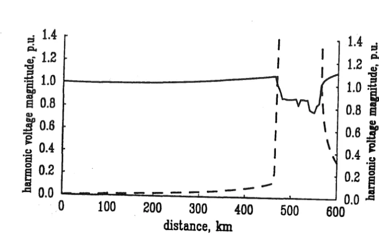
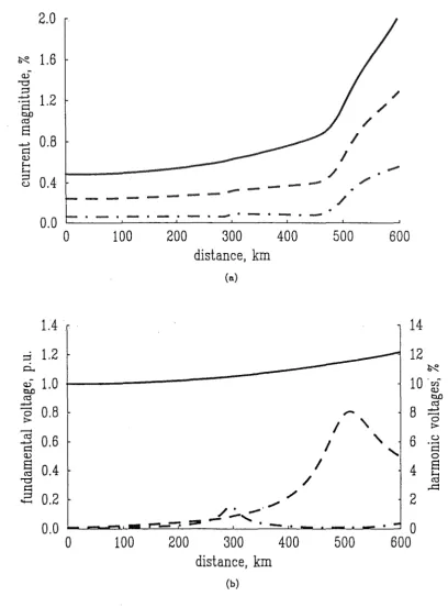
Line geometry for example 1 . . . . Harmonic voltage at the sending end of the line . . .

Layout and equivalent circuit of a non-homogeneous long distance transmission line. Harmonic voltage magnitudes at the receiving end of the compensated line . . . Standing waves along the compensated line of example 3 . . . . Standing voltage waves for the compensated line of example 3 together with the har-monic order to produce three-dimensional plots as observed from different positions Structure of the Jacobian-admittance matrix corresponding to a radial system. New Zealand grid below Roxburgh . . . .

A full cycle of the voltage waveform existing at: . A.1 Transmission line . . . .

B.1 Harmonic voltage magnitude for a single phase line above a lossy ground. B.2 Harmonic voltage magnitude for a double phase line above a lossy ground B.3 Harmonic voltage magnitude for a three phase line above a lossy ground

Bo4 Harmonic voltage magnitude for three single phase lines in parallel

96 98 · 103 · 106 .106 107

108 113 · 115 116 125 128 · 129 · 130 · 131 C.1 Transposed line diagram and equivalent 7r sections . . . 132 C.2 Diagram of terminal conditions . . . 133

C.3 Fundamental frequency three phase voltages at the end of the test line (open circuited) versus line distance . . . 135

Co4 Three phase third harmonic voltages at the end of the test line (open circuited) versus line distance . . . 137

C.5 Results of C-4 expanded at the region of resonance . . . 138

C.6 Fundamental a,

f3

and ground mode voltages at the end ofthe test line (open circuited) versus line distance . . . 139

(8)

C.S Fundamental Q ,

f3

and ground mode voltages at the end of the test line including two

sets of transpositions. . . 141 C.9 First and second resonant peaks of a 300 km line with . 142 C.lO Three phase voltages along the compensated line with . 143 E.1 Three unconnected single phase transformers

E.2 Grounded star : grounded star connection E.3 Star: star connection . . . . ..

E.4 Delta: delta connection . . . . . E.5 Grounded star: delta connection

(9)

List of Main Symbols

1/J,X

i,y 6.I,6.Y 6.V,6.U IN,YN

[G],[F],[H]

{Y}t,{Yi}

{Y}

[Z]

[1/J ]

[Tv],[Ti]

[YJ]

Zc

T

h

Magnetic fluxes Magnetizing currents

Vectors of superimposed harmonic currents Vectors of superimposed harmonic voltages Norton equivalent current sources

Matrices of magnetic admittances

Diagonal matrices of leakage admittances of transformer Diagonal matrix of transfer admittances of the line Lumped series impedance matrix of a multi conductor line Matrix of potential coefficients

Matrices of modal transformations

Harmonic admittance-Jacobian matrix of the entire network Characteristic imped3:nce

Propagation characteristic Length of the line

Harmonic order

Coefficients for the evaluation of ground impedances

(10)

The present research has given place to the publications cited below:

J. Arrillaga, E. Acha, T.J. Densem and P.S. Bodger. Ineffectiveness of transmission line transpositions at harmonic frequencies. Proceedings lEE Part C, 133(2):99-104,March 1986.

A. Semlyen, E. Acha and J. Arrillaga. Harmonic Norton equivalent for the magnetizing branch of a transformer. Proceedings lEE Part C, 134(2):162-169, March 1987.

A. Semlyen, E. Acha and J. Arrillaga. Newton-type algorithms for the harmonic analysis of non-linear power circuits in periodical steady state with special reference to magnetic non-linearities. In PES Winter Meeting, IEEE Power Engineering Society, New Orleans, Louisiana, November 17 1987.

J. Arrillaga, E. Acha, N. Watson and N. Veale. Ineffectiveness of transmission line VAR compensation at harmonic frequencies .. Accepted for presentation in ICHPS-IEEE to be held in Nashville, Indiana in September, 1988.

E. Acha, J. Arrillaga. Modal analysis of harmonic propagation with particular reference to the effect of transmission line transpositions. Accepted for presentation in ICHPS-IEEE to be held in Nashville, Indiana in September, 1988.

(11)

Abstract

Magnetizing harmonics in power systems have received limited attention. The general belief is that they do not reach harmful levels in interconnected networks. Moreover the modelling of non-linearities is not a straightforward procedure and so there has been little motivation to develop appropriate methodologies that allow a thorough investigation to take place.

In this thesis the problem of magnetizing harmonics in power systems is investigated. The results obtained show that, contrary to expectations, magnetizing currents can give rise to a considerable harmonic distortion in the voltage wave form of power networks operating under loaded conditions.

The method adopted in this research linearizes each magnetic non-linearity around a base operating point. The linearization exercise takes place in the complex-conjugate harmonic space and the individual linearized equations may be interpreted as harmonic Norton equivalents. These equations combine easily with each other and with the transfer admittances representing the linear part of the network. The overall process of linearization may be seen as a linearization of the entire network and can also be interpreted as a multi-nodal, polyphase harmonic Norton equivalent.

This problem is non-linear and the harmonic solution is reached by an iterative process. A re-linearization of the network takes place at each iterative step and so the solution is found through a Newton-type procedure. Several iterative strategies are tested, including unified and sequential solutions with either single or multi-evaluated Jacobians.

(12)

Acknowledgements

It is true that even a modest contribution, such as the present one, could not have been possible without a pleasent enviroment and the excellent resources provided by the University of Canterbury. Equally important has been the support and advice given by many people. In particular, I wish to thank Professor J osu Arrillaga, who has been a cornerstone in the development of this work. At a very early stage in this research I was also also fortunate to work under the guidance of Professor Adam Semlyen. The knowledge gathered during that brief period has proved to be the backbone of this thesis. I wish to extend my warmest thanks to Professor Semlyen.

Much earlier, at the beginning of my professional education, Salvador Acha pointed out power engineering to me as an area of rewarding endeavours. He also taught me many of the basic concepts that have been useful resource when dealing with the intricacies of this research. I hope the time is correct and this space is appropriate to express my gratitude to him.

The generous help of M.G. Derrington is truly appreciated. His detailed reading of the first part of the manuscript resulted in changes that have greatly enhanced the presentation of many of the arguments contained in this thesis.

(13)

Chapter 1

Introduction

1.1

General

The last quarter of the nineteen century saw the development of the electricity supply industry as a new, promising and fast growing activityl. Since that time electrical power networks have undergone immense transformations.

Owing to the relative safety and cleanliness of electricity, it quickly became established in man's environment. Nowadays it is closely linked to primary activities such as industrial production, transport, communications and agriculture. Population growth, expectations of higher standards of living, technological innovation and higher capital gains are just a few of the factors that have maintained the momentum of the power industry.

Clearly it has not been easy for the power industry to reach its present status. Throughout its development innumerable technical and economic problems have been overcome, enabling the supply industry to meet the ever increasing demand for energy with electricity at competitive prices. The generator, the incandescent lamp and the industrial motor were the basis of the success of the earliest schemes. Soon the transformer provided a means for improved efficiency of distribution so that the generation and transmission of alternating current over considerable distances provided a major source of power in industry and also in domestic applications. More recently the power converter has permitted the transmission of a large amount of power over very great distances, and the interconnection of individual systems having different frequencies.

Under ideal operating conditions the electrical wave of AC networks is expected to be sinu-soidal with constant amplitude and frequency. In practice, however, to a greater or lesser extent, all power plant components possess the undesirable property of distorting the electrical wave from its ideal sinusoidal form. This phenomenon, known as harmonic distortion of the wave form, has been aggravated by the number of electrical loads capable of producing considerable wave distortion. These include all forms of electric transport, arc-electric lamps, metal reduction devices and, more recently, the thyristor which, owing to its versatility and economy, has flooded the industrial and domestic markets [Gauper,Harnden and McQuarrie 1971].

Various adverse effects have been traced to the existence of non- sinusoidal waves. The most common being additional losses in the system, reduction in the useful life of power plant equipment, ill-tripping of protection devices, ripple spill-over and interference in communication circuits by power lines.

The problem of harmonics in power systems is not new. It is as old as the power network itself and the first reports can be traced to the beginning of this century [Clinker 1914] when transformers were the major source of harmonic distortion. Interference in communication circuits by power lines was the first problem which indicated the necessity of reducing the harmonic content of electrical waves.

lThls development took place in both Europe and The United States, simultaneously.

(14)

In spite of the inadequacies of measuring equipment and computation facilities, reductions in harmonic distortion were achieved through a series of practices such as the use of different three phase transformer connections, phase transpositions, the use of filters and improvements in transformer designs. Furthermore, communication equipment less susceptible to noise was developed, the circuits were insulated and different rights of way were chosen wherever possible. These remedies were sufficient, for example, to reduce the telephonic interference to tolerable levels.

The measures adopted were both technically and economically successful thanks to the op-erational and structural properties of the early electric networks. Low opop-erational voltages, radial systems. and short-distance transmission lines produced a low degree of imbalance and made the excitation of an harmonic resonance difficult. The harmonic sources of that time could only pro-duce low order harmonic injections, generally up to the thirteenth harmonic. Such is the case of saturated transformers, electric machinery connected to unbalanced circuits and rectified loads for electric traction purposes [Joint committee on electromagnetic interference 1914].

From the point of view of the supply industry the problem of harmonic distortion of the electric wave was considered to be solved and a phenomenum of the past. For several decades the problem was forgotten and practically no serious research was reported. It was regarded, if at all, as a purely academic exercise.

For most practical purposes the electrical wave was considered to be sinusoidal and the quality of the electrical energy delivered to the consumer was measured only in terms of constant voltage magnitude and constant frequency.

More recently, however, the design and operating conditions of modern power systems have changed radically. Owing to the very high voltages required to transmit the large amount of electrical energy demanded, the network has· suffered extreme imbalance. Furthermore, the technological innovations of our time have created new and more powerful sources of harmonic. The distortion of the waveform has reappeared as a problem having practical significance. This time, however, the picture appears to be considerably more complicated than in the past. The new sources of harmonics generate both low and high order harmonics and the resonant points are difficult to estimate because of the highly interconnected nature of modern networks.

The use of power semiconductor devices and modern appliances has grown very rapidly indeed and this, coupled with the traditional sources of harmonics and the proliferation of DC links has become a real challenge to the power engineer who has to operate and supply electricity to a large and varied number of devices characterized by their risk of causing major harmonic distortion into the network [Emanuel 1977].

Very little progress has been made in finding new remedies for the problem; the methods used at the beginning of the century are the same utilised today. However in this occasion extreme care must be exercised when such measures are applied. Large imbalance, continuous expansion of the network and tight interconnection may reduce their effectiveness. Moreover, due to the higher voltages involved, costs have also increased and those measures may consume an important proportion of the overall investment [Robinson 1966].

Because of its implications the problem has attracted the attention of both the supply in-dustry and the large consumers. Several countries have adopted regulations to limit the permissible level of harmonic distortion [Bradley,Morfee and Wilson 1985]

Significant progress has been made in the development of accurate and versatile instrumen-tation to monitor the harmonic behaviour of the network at the point of measurement, thus enabling effective enforcement of the legislation [Arrillaga 1981].

Measurements, however, become increasingly difficult to coordinate and increasingly expen-sive as the number of points simultaneously monitored increases [Breuer et al 1982].

(15)

Simulation, based on modern digital computers and powerful numerical techniques, provides answers which satisfy some of the requirements. A considerable effort has being devoted worldwide over the last ten years to finding the answer and several approaches which represent the problem more or less accurately have been reported but no solution so far put forward copes with it satisfactorily in all its complexities.

On one hand, transient studies and dynamic models for most ofthe power system components are already well advanced and, in principle, they could be used to determine the harmonic solution of the network [Dommel1969]. In practice the technique is rendered impractical for determining the harmonic solution because of the computational burden which arises when a large range of conditions is required or an interactive environment is sought. On the other hand, steady state solutions using harmonic phasor analysis have emerged as the natural alternative. A great deal of experience has been accumulated in the fundamental frequency solution of very large non-linear systems. Highly efficient numerical techniques of the Newton-Raphson type, together with sparsity and diakoptics facilities, have enabled the solution of large networks in a matter of seconds.

These developments have encouraged a similar line of thinking for harmonic analysis. How-ever, the problem undertaken is not a straightforward extension of the practices in current use at the fundamental frequency but is one of a more general philosophy and a greater degree of complexity.

Conventional studies are formulated on the premise that the sources are the system genera-tors. When viewed in the harmonic perspective, however, they behave as sources at some harmonic frequencies (among them the fundamental) and as sinks at other harmonic frequencies and, in gen-eral, they will act as harmonic frequency converters [Semlyen,Eggleston and Arrillaga 1986]. This is a change from tradition as power plcwt components such as the static converter and the power transformer which Were seen as loads at fundamental frequency analysis are now seen in harmonic operations in a dual source-sink role.

Transmission lines do not exhibit these properties. they act as passive admittances that vary with frequency in a non-linear fashion. Lumped transmission line models based on the nominal pi concept are no longer valid when dealing with harmonic frequencies, and long-line effects have to be incorporated. Moreover, modern power transmission lines are very unbalanced and the unquestioned practice of transposing the line as a means of restoring geometrical balance could not only render ineffective but also deteriorate further the symmetry of the harmonic voltages at the far end of the line [Arrillaga,Acha,Densem and Bodger 1986].

The accurate and reliable harmonic solution of a power system network incorporating all the above and other important effects requires the development of a new generation of mathematical models for all the power plant component. Scattered contributions to this developments have ap-peared in the technical literature recently and the research program of this department can be seen to be an important contribution towards the understanding and solution of problems which are of paramount importance to the present and future of the electrical power industry, worldwide.

(16)

Power transformers have long been the subject of widespread research. Early studies were largely confined to qualitative discussions drawn from practical observations and more recently, pas-sive harmonic models have been proposed. In practice, however, the magnetic core of the transformer is an active source of harmonic generation. It has the property of acting simultaneously as both har-monic source and sink. Moreover, it is not possible to anticipate particular values or limits in the amount of magnetizing current that a transformer can draw, as this is critically dependent on the magnitude and waveform of the excitation voltage and the quality of the transformer core.

Thus, a realistic transformer model suitable for power system harmonic analysis should not only incorporate voltage and frequency dependent effects, but also take proper account of the elec-trical connection and ability to combine easily with the external network.

Transformer models incorporating all these features are presented for the first time in this thesis. A parallel development to the harmonic Norton equivalent presented in this thesis models the transformer as a set of harmonic current sources [Dommel,Yan and Shi-Wei 1986].

Due to its characteristic as a very heavy distorter, the static power converter has received a great deal of attention and, although establishing accurate harmonic models for the converter taking due account of its control parameters is not an easy task, an outstanding model which rep-resents the converter as a set of harmonic currents is in active use [Yacamini and De Oliveira 1980]. Also a way of representing the static converter in the complex harmonic space has been reported [Mizuma,Sagisaka,Neri andSekine 1985].

Serious attention has recently been given to the synchronous generator [Semlyen,Eggleston and Arrillaga 1986] and [Mizuma,Sagisaka,Neri and Sekine 1985]. It behaves as an active source of harmonics both when supplying an unbalanced network and when operating in saturated conditions. The former case involves a harmonic conversion process between the stator and the salient poles rotor and is a function of both the degree of saliency of the rotor and the degree of unbalance of the external network.

Successful models which include the mechanism of harmonic conversion and which take place in the complex harmonic space are already available. Furthermore, harmonic studies of the interaction generator-converter have been reported.

1.2

Main aims

The main objectives of the thesis are:

1. To formulate new mathematical tools for the periodic, steady state solution of non-linear, dynamic circuits described by ordinary differential equations.

2. To develop harmonic, three phase transformer models which represent correctly the voltage and the frequency dependent effects of the magnetic core as well as the electrical connection. Furthermore, they should combined easily with the external network.

3. To improve both the versatility and the efficiency of present harmonic transmission line models and to investigate the behaviour of non-homogeneous transmission lines at harmonic frequen-cies.

(17)

1.3

Chapter Presentation

The material studied in this research project is organized as follows:

Chapter 2 introduces the concept of non-linear, steady state relationships into the harmonic analysis and discusses its suitability in modelling magnetic non-linearities of the transformer type. It also gives guidelines for the modelling of other power system elements amenable to similar treatment.

Although it is not explicitly mentioned as such, the approach to the harmonic modelling of power network elements on the basis of their input-output behaviour is already a favoured approach. Some elements of the system such as power converters are described by analytical equations which allow their response to be determined. Some other elements, however, may not have such equa-tions available and alternative ways of quantifying their response have to be established. Magnetic non-linearities are in this category but, fortunately, the relevant information is contained in their associated experimental magnetizing characteristics.

A clear understanding of the mechanics of magnetizing characteristics is essential when mod-elling power transformers. Magnetizing characteristics depend critically on the excitation voltage and they contain one part which is frequency dependant and another which is frequency independent. Chapter 3 Presents a linearization procedure that takes place in the real harmonic space and is suitable for determining the periodic steady state response of a class of non-linear circuits.

This is a more restricted development than the formulation presented in the next Chapter, because it is strictly valid only for cases of sinusoidal excitation plus a DC term. In practice, however, it has been shown to work well under cases of non-sinusoidal excitation.

Chapter 4 presents the derivation of new and efficient mathematical techniques for the harmonic solution of non-linear circuits subjected to periodic excitations.

The formulation is based on incremental linearization, which take place in the complex-conjugate harmonic space. The linearized model is not related to discretization in the time domain.

It is valid for any length of time as steady state solution. It is approximate because of the truncation of higher order terms in the process of linearization. It provides, however, a mean for the iterative solution of the circuit in a steady state by use of a harmonic Newton-Raphson method. After convergence, the harmonics will be in balance.

Chapter 5 develops three phase transformer models suitable for determining the steady state response under any kind of periodic excitation.

The magnetic circuit of the transformers is well modelled by using the technique of lin-earization in the complex-conjugate harmonic space. The double philosophy of operation source-sink and voltage and frequency dependence effects are included correctly. Moreover, the resultant three phase linearized model combines easily with the electric circuit of the transformer, and also with the external network.

Chapter 6 proposes alternative transmission line models that, owing to their versatility and reduced time of response, are suitable for interactive analysis of power system. Furthermore, it shows how linear elements also can be modelled in the complex conjugate-harmonic space.

(18)

Harmonic transmission line models based on transfer functions, rather than the equivalent pi concept are shown to be more efficient. New formulae for the frequency dependant part of the line are also proposed. These formulae are shown to be the fastest to date yet maintain a high degree of accuracy, and, coupled with the transfer function approach, provide the means for an interactive solution.

Chapter 7 presents the complex-conjugate harmonic space as a new frame of reference where, in principle at least, all the plant components of the power system can be framed. It offers a more general frame than the one provided by the phases and it is intended, only, for the harmonic analysis of power systems.

Here the harmonic space concept is further extended so that any number of multi-phase busbars can be accommodated. The resultant harmonic matrix equation couples all the busbars, phases and harmonics present in the network. Furthermore, any number and type of both linear and non-linear plant components represented by either a harmonic Norton equivalent or a harmonic admittance can be framed into it.

(19)

Chapter

2

Non-linear Excitation-Response

Relationshi ps

2.1

Introduction

Power networks are built up from a large number of elements of widely different natures and it may not be practical from a system point of view to establish harmonic models based on a detailed representation of their internal behaviour. On the other hand, all of them are amenable, in principle at least, to a nodal terminal description in the form of either a harmonic transfer admittance or a harmonic Norton equivalent. Linear components are modelled by transfer admittances while non-linear components are represented by ::.rorton equivalents. This philosophy of modelling relies on the assumption that means exist for quantifying the responses of each of the elements.

Some non-linear components, such as static power converters, have explicit equations associ-ated with their responses [Yacamini and De Oliveira 1980]. Other non-linear elements, however, may not have explicit equations. Magnetic non-linearities, for instance, belong to the class of elements for which analytical solutions are only feasible in a very restricted number of cases. Nevertheless, numer-ical solutions based on their steady state magnetizing characteristic are possible and are completely general. Both approaches to the problem are presented in this chapter.

Magnetizing characteristics are central to the harmonic solution of magnetic non-linearities and an overview of their physics, along with experimental ways of recording them, is presented in this chapter. In addition, analytical and numerical algorithms which may be used to calculate the harmonic currents and the magnetic admittances from the magnetizing characteristics are given.

2.2

Excitation-Response Characteristics

Consider the power plant component shown in figure 2.1, where only a single port is available for both the excitation and measurement of a response.

+ POWER

x(f) PLANT

COMPONENT

(20)

When a periodic,sinusoidal excitation x(t) is placed across the terminals of the plant com-ponent a periodic response

y(t)

takes place which could be either sinusoidal or non-sinusoidal. A sinusoidal response will be produced by a plant component with linear impedance and a non-sinusoidal response will be produced by a plant component with non-linear impedance.

Furthermore, the excitation-response characteristic of the plant component can be determined by supplying both the periodic excitation and the periodic response to any suitable device, e.g. an oscilloscope. The general characteristic exhibited by a linear power plant component is an ellipse, as shown in figure 2.2, which can degenerate into a straight line.

y

x

Figure 2.2: General x-y characteristic for a linear component

2.2.1 Idealized characteristics

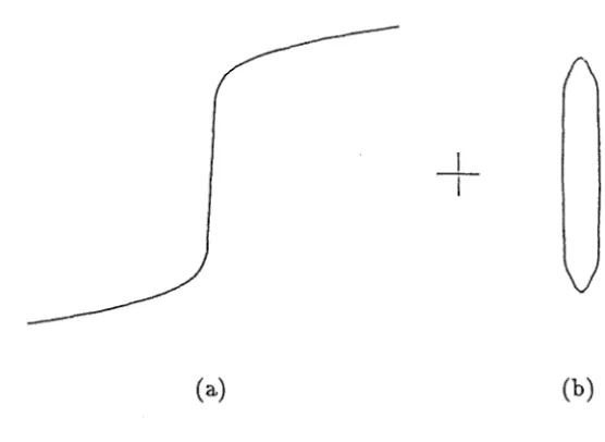
The response associated with most of the non-linear elements of the power system is difficult to determine by analytical calculations, except for very simple and idealized cases. For instance, the non-linear response of a lossless ferromagnetic core acting under moderate saturating conditions can be adequately represented by a polynomial equation, as shown in figure 2.3 (a).

I(t)=a"/t+b"/tn

+

'1jI (t)

lossless core

(a)

varying: band n

L----,>

--+--~

(b)

Figure 2.3: Polynomial characteristics corresponding to lossless cores (a) Schematic representation (b) Idealized characteristics

It will be shown in a later section of this chapter that the coefficients a, band n are determined

(21)

The static power converter acting under sinusoidal AC voltage excitation, infinite DC in-ductance and zero reactance on the AC side, presents another example of an idealized case. If the DC side current is free of harmonics, the AC line currents (the response) will consists of a series of rectangular blocks of current. In that case the response can be expressed conveniently by the series shown in figure 2.4 (a), while figure 2.4 (b) shows the excitation-response characteristic.

I(t)

+ vet)

i(t) = 4Idc X;l... sin(M) coa(hc.Jt)

1f h h 2

h-1.J.S •..•

v

'---_>

1 ,

-x = 0

ce

L = OJ

de

(a) _(b)

Figure 2.4: v-i characteristic for one phase of the static power converter ( a) Schematic representation (b) idealized characteristic

2.2.2 More realistic characteristics

When more realistic conditions are considered, the excitation-response characteristics of the non-linear power plant components will differ from those given above.

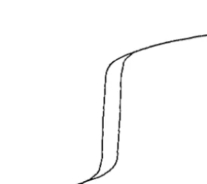
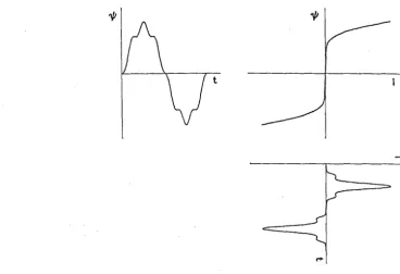
[image:21.566.201.350.536.668.2]

The characteristics of ferromagnetic cores will exhibit a looped form if there are losses. Figure 2.5 shows the looped characteristic resulting from plotting, point by point, a given sinusoidal excitation and the corresponding non-linear response.

(22)

The AC system to which the static power converter is connected will contain a certain amount of reactance rather than the zero value assumed for the idealized case of figure 2.4. This reactance, termed commutating reactance, plays an important role in the operation of the converter and its overall effects are to reduce the harmonic content of the current drawn by the converter [Arrillaga 1983] and to turn the idealized circuit of figure 2.4 into a lossy one.

Figure 2.6 (a) shows the v-i characteristic for one phase of the static power converter. It has been obtained by plotting a sinusoidal voltage and the current shown in figure 2.6 (b).

(a) (b)

Figure 2.6: v-i characteristic of a converter including commutating reactance effects (a) Lossy characteristic (b) A full cycle of the current

A more realistic characteristic can be obtained by considering a static power converter connected to a DC link with a finite amount of inductance. The v-i characteristic is shown in figure 2.7 (a), while figure 2.7 (b) shows the cycle of current being drawn by the converter.

(a) (b)

(23)

2.3

An Overview Of The Magnetizing Characteristic

2.3.1 The non-linear effects

Three non-linear effects are introduced by ferromagnetic cores, namely, saturation, hysteresis and Eddy currents. These three effects are exhibited by the magnetizing characteristic shown in figure 2.8, which corresponds to a small transformer and was obtained with a 50 Hz, sinusoidal

&iliilioo. '

.... / .... / .... / .... LJ· ..

·1 .. .. .... .. .. , ....

'

-1-1-1-1

... l ...

+ - 1 - - '

_{1 ....}₁

1

_· I-I-'-t-r--t ,--. t-r--t-,---

,'" ""F'" ''''F

l"·' ".

"'r' "',

1 1 1

I

-I-I-i=t~':':::';

.-:::.:: " ..

_-f

~=+---l

-rH-"-I-H_:-:l-:-:~H-t~:-:{+"

,...+-

'-:+tL:~-tL~-II~+H-IL~+11

~ +. . _t + + oj

- - - + - - + - ,

~i'

' + +

-1 -1 -1

""'1""~:'J" ,:_"7 ~:"J-'~~"'I"'"

I I

1

r"'T"""'T''''': .. "l"'''''T''''

I

- - - L - - - ' - - . - - ' - - - - ' - - - - L _ _ _

" " 1 " " " " ...

.~!~

....

1

.... 1

.... LI

1 " . .

I'

"~,-,,

",-

.. :

"~r~~-:-I-"

.. ,-.. ,',-

.. ,,' ....

Figure 2.8: Magnetizing characteristic recorded in the laboratory for a transformer of small rating

The magnetizing characteristic above can be divided into two main components, as shown in figure 2.9.

(a)

I

-,-(b)

Figure 2.9: Main components of the magnetizing characteristic (a) Characteristic of a lossless core (b) Loss cycle

[image:23.561.138.416.464.667.2]

(24)

The hysteresis phenomenom consists of two parts, a part which is frequency independent and is attributable to domain wall movements, non-magnetic inclusions and imperfections [Boon and Robey 1968] and a part which is frequency dependant and is refered to as the anomalous losses [Brailsford and Fogg 1964]. Losses associated with hysteresis are expected to be small in modern power transformers. Eddy currents, on the other hand, are not present when very slow (essentially zero frequency) traverses of the loop occur but any increase beyond zero frequency will give rise to Eddy currents which increase the loss per cycle. At power frequencies and above, this effect can account for two to three times as much loss as hysteresis does [Swift 1971].

2.3.2 Experimental magnetizing characteristics

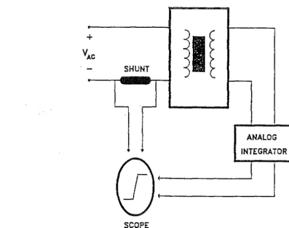
The experimental magnetizing characteristics of transformers of small rating can be recorded in the laboratory by means of the arrangement shown in figure 2.10.

SHUNT

n

-ANALOG INTEGRATOR

0t:

[image:24.562.93.383.263.492.2]

-SCOPE

Figure 2.10: Basic arrangement for the recording of magnetizing characteristics

The method is approximate because the voltage drop due to the resistance of the windings is not accounted for. It is based on a changing current being applied to one winding while the instantaneous voltage appearing across a second winding is integrated to determine the flux linkage. Both current and integrated voltage are supplied to either an oscilloscope or an X-Y plotter and the magnetizing characteristic is recorded.

The basic circuit in figure 2.10 can be modified to allow for greater accuracy and versatility. For instance, the resistive drop can be taken into account and, if voltage and current measurements are carried out in the same winding, the technique can be applied to both transformers and reactors. Furthermore, a digital integrator can be used instead of the analog one [Calabro,Coppadoro and Crepaz 1986].

(25)

A practical alternative lies in the use of a reversible DC supply rather than an AC source [Dick and Watson 1981]. This method can be seen as excitation by very low frequency AC whereby high flux levels can be obtained with the application oflow voltage and low power. Magnetizing char-acteristics measured using this approach will include saturation correctly and most of the hysteresis effect but their loss cycle will be very narrow. This is particularly true for ferromagnetic cores built of high quality materials. The reason for narrow loops is that neither Eddy currents nor anomalous losses are included.

Figure 2.11 shows the positive half of an experimental magnetizing characteristic for a modern three phase 25 MVA, 110/44/4 KV, Y/Y/D power transformer measured using DC excitation [Dick and Watson 1981].

1.2

1.0 :;; ':0.8 >( •

::J

;;:

,g 0.6.

'"

c

Ol

~ 0.4

0.2

Figure 2.11: Positive half of an experimental magnetizing characteristic of a modern three phase power transformer

2.3.3 Polynomial magnetizing characteristics

Finding analytical expressions to describe experimental magnetizing characteristics has been an area of active research [Hale and Richardson 1953]. Fitted polynomial and exponential equations containing a large number of terms have been proposed to represent lossless magnetizing characteris-tics [De Carvalho 1984]. Alternatively, a simple procedure suitable for a class of harmonic distortion problems is possible.

A fitted polynomial equation of the form

(2.1)

is determined, with the coefficients a, band n being derived from the following basic information,

corresponding to the lossless magnetizing characteristic:

• Coordinates of the knee

(26)

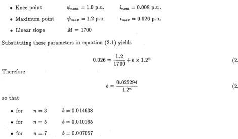
For example, a polynomial fitting for the magnetizing characteristic of figure 2.11 is shown below. The coefficients of the polynomial are taken from the experimentallossless curve as follows:

III Knee point 'if;nom = 1.0 p.u. inom = 0.008 p.u.

III Maximum point 'if;max = 1.2 p.u. imax

=

0.026 p.u.

III Linear slope M = 1700

Substituting these parameters in equation (2.1) yields

Therefore

so that

• for • for

III for

n=3

n=5

n=7

b

=

0.014638

b = 0.010165

b

=

0.007057

0.026 =

1~~0

+

b X 1.2n

b = 0.025294 1.2n

(2.2)

(2.3)

The selected magnetizing characteristic requires a current i

=

0.008 when 'if;

=

1 and therefore

n

=

7 is the best approximation. The chosen fitting is then [image:26.559.33.504.99.374.2]

i

=

17~0

+

0.007059 'if;7

(2.4)

Figure 2.12 compares the actual transformer magnetizing characteristic with that obtained by the polynomial of equation (2.1). They are shown to be in good agreement in the region 0 :s:; 'if; :s:; 1.2 p.u.

1.2

.!:! 0.6

Q;

co

'"

~ 0.4

0.2

polynomial experimental

(27)

2.4

Derivation Of The Harmonic Information Of Magnetizing

Char-acteristics

2.4.1 Analytical representation of the magnetizing characteristic

It was shown in the previous section that an experimental magnetizing characteristic can be

approximated by the polynomial form

(2.5)

where n is an odd integer. Since equation (2.5) has odd symmetry, the magnetizing characteristic

can be well fitted to experimental curves by noting that

II the coefficient a corresponds to the initial slope

II the exponent n is a measure of the sharpness of the knee II after a and n have been selected, the coefficient b can be

ob-tained so that the curve passes through the point i

max , 7/Jmax

Once the coefficients a, band n have been found, Equation (2.5) is evaluated at a particular

base operating flux

7/Jb,

(2.6)

and also its derivative,

(2.7)

It must be noted that

(2.8)

which can be expanded into

m

7/J'b

=

7/J'b:max

2),B~ sine

iwt)

+

,By

cos(

iwt»

(2.9) i=O

where

(2.10)

To obtain equation (2.9) consider the more general expression

m

(sin(x)+a)m = :LC~am-lsinj(x)

(2.11)

(28)

The binomial coefficients

cln

are given below arranged in the triangle of Pascal to show how they can be calculated recursively:

1

1 1

1 2 1

1 3 3 1

1 4 6 4 1 (2.12)

1 5 10 10 5 1

1 6 15 20 15 6 1

1 7 21 35 35 21 7 1

etc

If the expression (2.12) is seen as a lower triangular matrix LI , then equation (2.11) can be

written as

(sin(x)

+

a)m = am X (row m ofLI) X diag{a-i } X col {sini(x)}

j = 0,1,2, ... The powers of sin( x) are given as

sino x

=

1 sinl x sin x

sin2 x

=

:2(1- cos2x) 1 sin3 x

=

~(3

sinx - sin 3x) sin4 x 8(3 -1 4cos2x

+

cos4x) sin5 x

=

11

6(10 sin x - 5sin3x

+

sin5x) sin6 x 32(1O-15cos2x 1

+

6cos4x - cos6x) sin7 x

=

614 (35 sin x - 21 sin 3x

+

7 sin 5x - sin 7 x)

(2.13)

(2.14)

It is noted that the coefficients in equation (2.14) can be obtained from the right half of the triangle in expression (2.12), split vertically. Moreover,they can be accommodated in a lower triangular matrix and change signs where appropriate:

I

'2 0 1 1 0 -1

L2

=

0 3 0 -1 (2.15)

(29)

Now equations (2.14) can be written as:

(2.16)

i = 0,2,4, ... , m - 1

j

=

0,1,2, ... ,m

Substitution of equation (2.16) into (2.13) yields

i = 0,2,4, ... ,m-1

j

=

0,1,2, ... , m

If a

=

0, equation (2.16) can be used directly. Both equations (2.16) and (2.17) can be written more simply:

sinm(x) = Cl X col { cos(ix)

sin((i

+

l)x) (2.18)

i

=

0,1,2, ... ,m

and

( . () _sm_x

+

_a)m _ _- _{C2 X}_co1 { _{sine (i}cos(

+

ix ) _l)x) (2.19)

i

=

0,1,2, ... ,m

where

(30)

2.4.2 Numerical example 1

For a given characteristic i = f('l/Yb) = O.0017/Jb + 0.0743'l/Y~ and 'l/Yb = sin(x) + 0:

(

(20:)3 ) (

t

(sin(x)+

o:?

=!

(1 3 3 1) (20:)2 0

4 (20:)1 1

(20:)° 0

1 ) (

Si~X

)

o

-1 cos2x (2.20)

3 0 -1 sin3x

and for the particular case when 0:

=

0.5 then

) (

1 )

sznx cos2x -1 sin3x

(2.21)

or

(sin(x) + 0.5)3

=

7/8 + 3/2 sin(x) - 3/4cos(2x) - 1/4sin(3x) (2.22)

and substituting into the polynomial characteristic,

i

=

f( 1jJ)

=

0.0655 + 0.11246 sine x) - 0.05573 cos(2x) - 0.01858 sin(3x) (2.23)

The harmonic content, in phasor form, is readily available from the above result,

Zdc = 0.0655

i1 = 0.0 - jO.11246 Z2 = -0.05573 + jO.O i3 = 0.0 + jO.01858

also

(sin(x) + 0.5)2

=

3/4 + sin(x) - 1/2 cos(2x) (2.24)

and

(31)

2.4.3 Point

by

point representation of the magnetizing characteristic

As an alternative, a full cycle of the magnetising current can be derived from the experimental magnetizing curve using discrete values of flux as shown in figure 2.13 and the derivative of the function i =

f(

7jJ) can be derived by numerical analysis.

t

Figure 2.13: Point by point derivation of magnetizing current from the fl1L,{ waveform and magnetizing characteristic

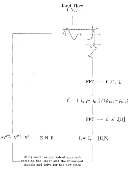
The current and derivative wave-shapes are then subjected to a fast Fourier transform. This procedure is the numerical version of the analytical solution based on equations (2.6) and (2.7). The solution requires the following steps:

1. A full period of the flux wave is impressed, point by point, upon the experimental characteristic 7jJ - i and the corresponding magnetizing current h(t) is thus determined in the time domain. 2. By means of the complex Fourier transform (FFT version), the magnetizing current

ib(t)

is solved in the frequency domain and the real and imaginary coefficients of the harmonic currents are obtained.

3. Using the magnetizing current and the magnetic flux, the derivative of the function i

=

f(

7jJ) is evaluated. [image:31.564.55.423.162.414.2]

(32)

2.4.4 Numerical example 2

Figure 2.14 (a) shows a full period of the magnetizing current resulting from impressing, point by point, a full period of the magnetic flux

'¢b

=

sin(wt)

upon the experimental magnetizing characteristic of figure 2.8 (reproduced here as figure 2.14 (b)).

( a) (b)

Figure 2.14: Current resulting from applying a sinusoidal excitation to a lossy transformer (a) A full cycle of the current (b) Magnetizing characteristic

An FFT exercise is applied to the above magnetizing current and the harmonic content is given below.

21 = 0.003669 - jO.033906

23 _{= 0.001365}

+

jO.018590 25 = -0.000514 - jO.005185 27 = -0.000466 - jO.000166 29 = 0.000251

+

jO.000202

211 = 0.000253

+

jO.000165

213 =-0.000110 - jO.000039

i15 =-0.000111- jO.000019

As expected, the magnitude of the harmonic content decreases rapidly with the harmonic order and, due to the symmetry of the excitation and the response, no even harmonics are present. For this level of the excitation it is observed that the real component of the harmonic content (losses) is significant when compared with the imaginary part and such significance increases with the harmonic order, although it decreases with the excitation level, e.g. i7 = 0.000563 - jO.003917

(33)

On the other hand, figure 2.15 (a) shows the resultant magnetizing current when a full cycle of the magnetic flux

'l/Jb

=

sin(wt)

is impressed, point by point, upon the lossless magnetizing characteristic of figure 2.9 (a) (reproduced here as figure 2.15 (b».

(a)

(b)

Figure 2.15: Current resulting from applying a sinusoidal excitation to a lossless transformer (a) A full cycle of the current (b) Magnetizing characteristic

The corresponding harmonic content is given below,

21 0.0 - jO.033906

i3 0.0

+

jO.018590

25 0.0 - jO.005185

i7 0.0 - jO.000166

29 0.0

+

jO.000202

i11 0.0

+

jO.000165

213

=

0.0 - jO.000039 215

=

0.0 - jO.000019

In this case the imaginary component of the harmonic content equals that involving the complete magnetizing characteristic but it contains no real part. It may also be observed that in the process of neglecting the loss cycle, the most important component of the higher order harmonics (real part) has been dropped. However, the magnitude of these harmonics is very small and it is unlikely that they will have a major effect in actual computations.

(34)

2.5

Conclusions

It was stated in the introduction to this chapter that, in principle, harmonic models for all the plant components of the power system based on the concept of excitation-response relationships, are possible. This philosophy of modelling avoids the complexities associated with the internal mechanisms of the power components and only requires them to have explicit equations, or other suitable means, for the description of their response.

The above approach is the one pursued in the present research and, aiming at this, some fundamental concepts have been presented in this chapter and the ground work has been prepared for the application of non-linear excitation-response characteristics to actual computations.

A wide range of both idealized and realistic characteristics has been presented for the trans-former and the static power converter. While magnetizing characteristics have been used by electrical engineers for almost a century, no attention has been paid so far to the characteristics of static power converters.

A probable reason is that converters possess explicit equations for the evaluation of their responses and thus their explicit v-i characteristic may play no role in actual computations. However, the use of converter v - i characteristics has been shown to provide greater insight into their steady state operation

On the other hand, it has been shown that ferromagnetic cores present the opposite problem but, in the absence of explicit equations, their response can be determined by using a suitable magnetizing characteristic which is usually derived experimentally.

Several techniques, with different degrees of accuracy, are available for the derivation of magnetizing characteristics. However, fl;om the three non-linear effects introduced by ferromagnetic cores, saturation is the effect that plays the major part in the harmonic distortion process.

Magnetizing characteristics contain the relevant information needed for the harmonic solution of magnetic non-linearities and analytical and numerical procedures have been presented here for the determination of both magnetizing currents and magnetic admittances.

The analytical approach, based on the Pascal's triangle, provides an elegant and easy way of extracting the relevant harmonic information from a polynomial representing the magnetizing characteristic. However, its range of applicability is limited to cases of sinusoidal excitation, plus a DC term, and its accuracy relies on the ability of the polynomial to match the lossless magnetizing characteristi c.

(35)

Chapter 3

The Real Harmonic Space

3.1

Introduction

An essential part of the computer-aided analysis of networks containing non-linearities is the evaluation of their steady-state response when subjected to a periodic excitation. This has been a topic of active research in the areas of circuit theory, control engineering and electronics over the last twenty years.

In principle, the periodic solution can always be found by integrating the differential equa-tions that describe the system until the transient response dies out; but this brute force approach becomes prohibitively expensive whenever the transients are governed by time constants that are much larger than the period of the driving force [Director and Wayne 1976].Nevertheless, integrating the differential equations was the first approach adopted for the solution of this kind of problems, partly because numerical integration techniques have been reasonably well known by most engineers over many years but also because an alternative solution was not straightforward to formulate [N akhla and Branin 1977]. It was necessary to carry the integrations for a considerable number of periods before the transient became small enough to be ignored. Clearly, better methods of solution were needed.

More efficient formulations, intended for electrical and electronic circuits, exist nowadays. In very general terms they can be classified into harmonic balance techniques, shooting methods and the describing function approach. The former two solve the problem to a specified accuracy level and are valid for cases of arbitrary (periodic) excitation.

Shooting methods take the approach of integrating the dynamic equations over one or two full periods and then solving the two point boundary-value problem by iteration. The methods are reported to be well-behaved and yield the initial state of the transient response in addition to the final harmonic solution. However, numerical integration of the dynamic equations is still required.

The harmonic balance technique is based on an iterative, steady state approach where each state variable is represented by a Fourier series that satisfies the requirement of periodicity. In order to ensure convergence, an optimization algorithm is used to adjusts the coefficients of the Fourier series. Thus, the system equations are satisfied with least error and with a minimum number of iterations. A number of examples corresponding to electronic circuits have been solved and in every case successful convergence was achieved with a smaller execution time than that required for the integration of the corresponding dynamic equations over two full periods [Nakhla and Vlach 1976].

(36)

In the past two decades, the determination of the periodic response of a non-linear networks has not been a problem of major concern for the power engineer. When the need for a solution first arose, methods based on the integration of the differential equations describing the non-linearity were used [Dommel1969].

Owing to the growing number of new and powerful harmonic sources being connected to the transmission grid as well as the traditional sources of harmonics the problem of evaluating the periodic response of power networks has now been acknowledged as a priority and ambitious research programs have been initiated, worldwide, to achieve it.

Non -lineari ties in power systems, as well as linear com ponen ts, are m ul ti -phase and frequency-dependant. In general, the problems they produce are more difficult to solve than their electronic counterparts. The solutions proposed for electric and electronic circuits are not always either suitable or directly applicable to the case of power circuits and although some of the fundamental ideas are similar, the problem of power system non-linearities must be addressed in a different way.

For most steady-state operating conditions the problem of power system harmonics can be viewed as one of a fundamental voltage with a superimposed ripple because the harmonic voltages existing in the network are only a few per cent of the fundamental.

Thus, when an iterative approach (harmonic balance technique) is adopted for the harmonic solution of the non-linear power system, the undistorted load flow solution provides a very good initial estimate of the final solution with harmonics. If no resonant conditions are involved the harmonic solution is reached in a reduced number of iterations (less than five), even if no optimization techniques are used to adjust the coefficients of the Fourier series. However, convergence problems are expected to occur when poorly damped resonances are present.

An algorithm, which exploits the points mentioned above, has been proposed recently [Dom-mel,Yan and Shi Wei 1986] and applied to the problem of magnetic non-linearities of the transformer type. It is a sequential iterative algorithm that models the transformer magnetizing branch as a set of harmonic current sources calculated from a point by point representation of the magnetizing characteristic. It uses nodal analysis to represent the linear part of the network.

Dommel's algorithm is very simple and represents a major step forward in the development of more efficient tools for the harmonic solution of non-linear power systems. However, the proposed algorithm is based on a Gauss-Seidel numerical procedure and, it is worth considering the development of an alternative model based on Newton-Raphson procedures.

In this research harmonic Newton-type algorithms have been developed that are suitable for the solution of both single and multi-phase circuits. They belong to the class of steady-state solutions and fully exploit the nodal analysis which has been used so successfully by power system engineers for most of their traditional studies. These formulations are based on local linearization as opposed to the describing function, which is based on global linearization and the process takes place in the harmonic space. Moreover, the resultant linearized equations may be interpreted as harmonic Norton equivalents that combine easily with the linear network in a unified frame of reference when that linear part is also represented in the harmonic space.

One of these formulations, to be presented in the next chapter, is valid for any kind of symmetrical or asymmetrical, periodic excitation and provides a solution to a specified level of accuracy. It takes place in the complex-conjugate harmonic space [Semlyen,Acha,Arrillaga 1987(a)]. The other formulation is presented in this chapter. In theory it has a more restricted scope because it is strictly valid only for cases of sinusoidal excitation plus a DC term. In practice, it can also be used for cases of non-sinusoidal excitation [Semlyen,Acha,Arrillaga 1987(b )].

(37)

This solution is based on linearization of the magnetizing characteristic around a base op-erating point using small increments of voltages and currents of the fundamental and harmonic fre-quencies. This permits the postulation (for guidance at this stage-proof is given in the next section) that the following linear equation exists:

I

=

Ib

+

[G]b.V

where I is the vector of resultant harmonic currents

Ib is the base vector of harmonic magnetizing currents

.6. V is the vector of superimposed harmonic voltages

[G]

is an admittance matrix to be derived from a given magnetizing curve

(3.1)

The variables I,Ib and .6. V include the increments offundamental frequency and have both a longitudinal component (Le. in phase with the base flux) and a transversal component (i.e. leading the longitudinal component by 900

) .

The multi-input/multi-output diagram of figure 3.1 shows a conceptual representation of equation (3.1).

Figure 3.1: Harmonic input/output relations in a non-linear device

3.2

Harmonic Norton Equivalent

3.2.1 General procedure

Given the magnetizing characteristic

i =

I( 1/J)

(3.2)

a base flux linkage is assumed

?/;b

=

1/Jb,max sine

wt)

+

1/Jdc (3.3) with an increment of small terms

00 00

b.1/J

=

I:

b.

?/;:nax,h sine

hwt)

+

I:

b.1/J':nax,h CoS(

hwt)

(3.4)

(38)

The resultant flux linkage is

(3.5)

so that i of equation (3.2) becomes, by a Taylor expansion around 'l/Jb truncated after the first order term,

i = I( 'l/Jb,max sin(wt)

+

'l/Jdc)

+

f'e

'l/Jb,max sin(wt)

+

'l/Jdc)b..'I/J (3.6)

In equation (3.6) both functions

I(

'l/Jb) and

f'e

'l/Jb) are periodic in t. Therefore they can be represented by Fourier series in sin(kwt) and cos(kwt). Substituting equation (3.4) into equation (3.6) yields:

00 00

2

=

L

1:nax,k sin(kwt)

+

L

1~ax,k cos(kwt)

k=l k=O

+

(t.

a~ax,isin(

iwt)

+

t.

a~ax,i

cos( iwt))

X

(f

b..'I/J:nax,h sin(hwt)

+

f

b..'I/J~ax,h

COS(hwt))

h=l h=O

(3.7)

Here the products of sine and cosine functions yield more sine and cosine functions so that the second term on the right hand side of equation (3.7) will have the form:

00 00

b..i

=

L

b..1:nax,h sine hwt)

+

L

b..1~ax,h cos( hwt) (3.8)

h=l h=O

If all current and flux linkage harmonics of equations (3.8) and (3.4) are assembled into the vectors

,6.1 = [ ... _,6.1'_max,k ...

I ...

b..I" _max,k .. .

]t

(3.9) ,6. .,. _'P

= [ ...

b.. 'I/J' _max,k ...

I ...

b..

.,,1/

_'+'max,k .. .

]t

(3.10)

then, comparing the coefficients in equations (3.7) and (3.8) corresponding to the same sine and cosine functions, yields

(39)

3.2.2 Matrix

[AJ

identification

The matrix

[A]

can be identified by taking all elements of the vector fl'lj; of equation (3.10) equal to zero, except one which is set to unity. Let this be fl'lj;'max h' Then in equation (3.7) the following multiplication is to be performed, '

00 00

(~=

ai

sin