Subgraph Matching Using Graph Neural Network

(1)

Subgraph Matching Using Graph Neural Network

GnanaJothi Raja Baskararaja, MeenaRani Sundaramoorthy Manickavasagam

Department of Mathematics, V. V. Vanniaperumal College for Women, Virudhunagar, India. Email: gnanajothi_pcs@rediffmail.com, smmeenarani@gmail.com

Received May 4th, 2012; revised August 1st, 2012; accepted August 8th, 2012

ABSTRACT

Subgraph matching problem is identifying a target subgraph in a graph. Graph neural network (GNN) is an artificial neural network model which is capable of processing general types of graph structured data. A graph may contain many subgraphs isomorphic to a given target graph. In this paper GNN is modeled to identify a subgraph that matches the target graph along with its characteristics. The simulation results show that GNN is capable of identifying a target subgraph in a graph.

Keywords: Subgraph Matching; Graph Neural Network; Backpropagation; Recurrent Neural Network; Feedforward Neural Network

1. Introduction

In many practical and engineering applications the un- derlying data are often represented in terms of graphs. Graphs generally represent a set of objects (nodes) and their relationships (edges). In an image, nodes represent the regions of the image that have same intensity or color, and the edges represent the relationship among these regions.

Subgraph matching has a number of practical applications such as object localization and detection of active parts in a chemical compound. Subgraph matching is mainly analyzed in object localization problem. For example in military areas to identify a particular object, say tank from a satellite photograph, the whole area can be converted into a graph with nodes having labels repre- senting color, area, etc. of the region. The subgraph which represents a tank can be made identified by subgraph matching. The suspected area to which a tank belongs can be restricted and the corresponding restricted graph can be considered for identification.

F. Scarselli, M. Gori, A. C. Tsoi, M. Hagenbuchner, and G. Monfardini have proposed a GNN structure which can be considered as an extension of recurrent neural network (RNN) to process very general types of graphs. The GNN model implements a function  that maps a graph G into an m-dimensional Euclidean space. The function depends on the node, so that the classification depends on the properties of the node. F. Scarselli, M. Gori, A. C. Tsoi, M. Hagenbuchner, and G. Monfardini have applied GNN to different types of problems such as Mutagenesis problem [1], subgraph matching problem

[1], Clique problem [2], Half Hot problem [2], and Tree depth problem [2]. A. Pucci, M. Gori, M. Hagenbuchner, F. Scarselli, and A. C. Tsoi [3] have applied GNN to the movie lens data set and have discussed the problems and limitations encountered by GNN while facing this particular practical problem. A comparison between GNN and RNN is made by V. Di Massa, G. Monfardini, L. Sarti, F. Scarselli, M. Maggini, and M. Gori [4] and they have shown that problem GNNs outperforms RNNs in an experimental comparision on an image classification.

In the subgraph matching problem discussed by F. Scarselli, M. Gori, A. C. Tsoi, M. Hagenbuchner, and G. Monfardini [1], the goal of the problem is to identify all the nodes of a larger graph which also belong to the con-sidered subgraph. In this paper, the trained GNN is iden-tifying a subgraph that matches the target graph along with its characteristics.

The structure of the paper is organized as follows: Section 2 describes GNN in the linear case, Section 3 explains subgraph matching problem, Section 4 gives the proposed algorithm for generating the graphs and identi-fying the subgraph in the training data. Experimental results and discussion are given in Section 5.

2. Graph Neural Networks

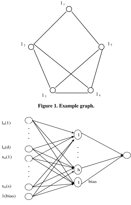
A graph G = (V,E), where V is a set of points called nodes, and E is a collection of arcs connecting two nodes of V. Let ne[n] be the set of nodes connected to the node

n by arcs in E. Figure 1 represents example graph with 5 nodes. The nodes of G are attached with random label

c n

lR . A state vector s n

(2)

which represents the characteristics of the node (i.e. adja- cent nodes, degree, label etc.). The state vector of a node with dimension s is computed using a feedforward neural network called Transition network which implements a local transition function fw.

   



, ,

n w n ne n ne n

x  f l x l



(1)



  , ,

u ne n

h_w l_n x_{u u}l







(2)

For each node n, hw is a function of the state, label of the neighboring node and its own label. Each node is associated with a feedforward neural network. Number of input patterns of the network depends on its neighbors. The hw is considered to be a linear function. When

,



, ,



,

w n u u n u u n

h l x l A x b b R_n sis defined as the output of feed forward neural network called bias network which implements w , ,

, n u sxs

:

 c s

R R b_n _w

 

l_n

A R is defined as the output of the feed forward neural network called forcing network which implements

,

2 2

: c s s

w R R

  _

 





, resize , ,

n u w n u u

sxne

A l x l

n

 _



where and resize operator allocates s2 elements in the output of forcing network to a s × s matrix.

 

0,1 

Let x, l denote the vector constructed by stacking all the states and all the node labels respectively of the graph. Equation (1) can be written as xF_w



x l,







. Banach fixed point theorem ensures the existence and the uni- queness of solution of Equation (1) in the iterative scheme for computing the state x t 1 Fw



 

,



.

x t l



, where x(t) denotes the tth iteration of x. Thus the states are computed by iterating

n w n ne n ne n This computation is interpreted as a recurrent network that consists of units namely the transition networks which compute fw. The

units are being connected as per graph topology.



1





 

, _{ }, _{ }

x t  f x t x l

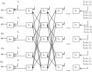
The output of each node of a graph is produced by a feedforward neural network called output network which takes as input the stabilized state of the node generated by the recurrent network and its label. For each node n, the output on is computed by the local output function gw as . Figures 2 and 3 represent output network and graph neural network correspondingly for the example graph.



, n w n n

o g x l

3. Subgraph Matching Problem

The subgraph matching problem is a computational task in which two graphs G and H are given as input, and one must determine whether G contains a subgraph that is isomorphic to H. In Figure 4, a graph G and a target graph H which is to be identified in G is given. H. Bunke [5] has demonstrated applications of graph matching by

l 1

l 2

l 3 l 4

l 5

Figure 1. Example graph.

ln(1)

ln(d)

xn(1)

xn(s)

1(bias)

1

h

1

. . .

[image:2.595.308.536.88.445.2]

bias

Figure 2. Output network.

giving examples from the fields of pattern recognition and computer vision. O. Sammound, C. Solnon, and K. Ghedira [6] have proposed ant colony optimization algo-rithm for solving graph matching problems and have compared with greedy algorithm approach on graph matching problems. D. Eppstein [7] has solved the subgraph isomorphism problem in planar graphs in linear time, for any pattern of constant size applying dynamic programming. C. Schellewald and C. Schnorr [8] have presented a convex programming approach for subgraph matching.

F. Scarselli, M. Gori, A. C. Tsoi, M. Hagenbuchner, and G. Monfardini [1] have used GNN to identify all nodes of subgraphs in larger graph which are isomorphic to target graph. In Figure 4, for the graph G a single in-put pattern is considered. As the graph G contains four subgraphs isomorphic to H, the GNN will identify all the nodes which are used to form the target subgraph. If this pattern is used for training or testing the GNN, the ex-pected output is a vector (0 1 1 1 1 1 1 0 1 1).

(3)

l1,x2, l2 l1,x5, l5

l2,x1, l1 l2,x3, l3 l2,x4, l4

l3,x2, l2 l3,x4, l4 l3,x5, l5

l4,x2, l2 l4,x3, l3 l4,x5, l5

…

fw

fw fw

fw

fw fw

fw

fw fw

fw

fw gw

gw

gw l1

l2

l3

l4 O1

O2

O3

O4

…

fw fw

gw O5

l5

[image:3.595.148.460.92.344.2]

l5,x1, l1 l5,x3, l3 l5,x4, l4

Figure 3. Graph neural network.

5. Find all possible nCm combinations of the n nodes of the graph G that form the subgraph H. For each possible combination,

8 3

7 4

5 2

6 1

9 10

G

1

2 5

4 3

H

1) Label the m nodes of the graph G by the label given to the nodes of H and the target of the corresponding nodes as 1.

2) Label the remaining n-m nodes with different random numbers and their corresponding target as 0.

(a) (b)

[image:3.595.59.294.107.489.2]

4.2. GNN Training Figure 4. Subgraph matching.

6. Initially assign the state vector of each node as zero vector.

generated. In each input pattern, a subgraph isomorphic to H is assigned node labels corresponding to H. Training or testing phase of GNN identifies nodes of a subgraph isomorphic to H for every input pattern. For the graph G expected output of the input pattern are (0 1 1 1 1 0 0 0 0 1), (0 1 0 0 1 1 0 0 1 1), (0 0 1 1 1 0 1 0 0 1), and (0 0 0 0 1 1 1 0 1 1).

7. Generate bias network with c input neurons, h hidden neurons, and s output neurons.

8. Generate single hidden layer forcing network with 2*c + s input neurons, h hidden neurons, and s*s output neurons.

9. Generate output network with c + s + 1 input neurons, h hidden neurons and 1 output neuron.

4. Training Algorithm

10. Assign weights randomly for all the network from

(0,1).

4.1. Preprocessing

11. Calculate output of the Transition network and bias network.

1. Generate connected graphs randomly with n number

of nodes say 1, 2 ··· n. 12. Compute state vector for each node of the graph using Equation (2).

2. Select a subgraph H with m nodes which is to be

identified in the graph G. 13. Repeat steps 11 and 12 until the state vector of each node is stabilized.

3. Label each of the m nodes of the subgraph H from a

set of random numbers. 14. Calculate output of the output network by feeding the stabilized states and label of the node as input and then calculate mean squared error.

(4)

15. Weights of all the networks are updated using backpropagation technique namely Generalized Delta rule.

16. Repeat steps 11 to 15 until desired accuracy is obtained.

5. Results and Discussion

The GNN model is developed using Matlab code. The network is trained and tested to match the subgraph on 5 nodes with graphs of 6 nodes to 10 nodes. Graphs are generated randomly with fixed number of nodes (n). Each pair of nodes in the graph are connected with some probability ( = 0.2). Each graph is checked for connec- tivity. If not connected, random edges between non ad- jacent nodes are added until the graph becomes connected. Select a random graph H on 5 nodes that is to be matched with the generated graph G. Label the vertices of H randomly from 20 to 30. The generated graph G may or may not have the subgraph H in it. A subgraph H is included in the generated graph G to assure the existence of the subgraph in G. A graph G may have more copies of H in it. They are identified by considering all possible nCm combinations of the nodes in G. The subgraph H may be present with different orientations in G. They are identified by considering all permutations of a possible m combination of the nodes of G. For all identified combinations the corresponding nodes of G are assigned the labels of the nodes of H and the target for these nodes are assigned 1. The remaining nodes are la- beled with random numbers from 1 to 15 and the target for these nodes are assigned 0. For all possible combination of n and m, each combination corresponding to a subgraph is taken as a separate input pattern and p denotes the number of input patterns.

In the example graph of Figure 4, a permutation 2 9 6 5 10 among the numbers given by the combination 2 5 6 9 10 form the subgraph given by H. The labels (20, 25, 21, 27, 24) (say) given to the nodes of H are correspondingly assigned to the nodes 2, 9, 6, 5, 10 of G. The corresponding target vector of G is (0 1 0 0 1 1 0 0 1 1). Another permutation of this combination namely 2, 10, 5, 6, 9 also forms the subgraph given by H and the label given to these nodes are 20 to node 2, 25 to node 10, 21 to node 5, 27 to node 6 and 24 to node 9. The corresponding target vector is also (0 1 0 0 1 1 0 0 1 1). Hence, the same combination forms different input patterns though the target vector is same.

The transition function hw and the output function gw are implemented by three layered neural networks with 5 hidden neurons. Sigmoidal activation function was used in the hidden and output layers of the network. This experiment is simulated for 5 different runs. In every run different p input patterns are generated and is used for training and testing, but first 30 patterns are considered

for validation. In this experiment, label dimension (c) is considered as 1 and state dimension as 2. Termination condition is fixed as mean squared error 0.1. The weights of the networks are initialized randomly from (0, 1). Value of  used in the function of the transition network is randomly chosen between 0 and 1. When the value is more than 0.5, there is the possibility of dividing by zero in calculating the state vector xn. Hence  is set as 0.005. The learning rate and momentum used in the generalized delta training algorithm are 0.1 and 0.01 respectively. The learning rate and parameter values are fixed by trial and error. The wrongly chosen values made the training diverge. In each run, the number of input patterns varied. The accuracy in terms of percentage is obtained for mean squared error value less than 0.1. Number of graphs and number of nodes of the graphs considered on each run and obtained results are tabulated in Table 1. The experimental results show that the time taken for convergence increased when the number of input patterns increased. Experimental results show that more than 96.5% of the graphs are identified correctly on each run.

6. Conclusion

[image:4.595.310.538.452.735.2]

GNN is modeled to find the desired subgraph with any orientation in a graph. Label, and adjacency of the nodes are used to represent the nodes of a graph as input to GNN. From all possible combinations and permutation

Table 1. Accuracies obtained for different nodes in G ma- tching with 5 node graph.

N _GraphsNo. of

No. of input patterns

Accuracy (%) Epoch Time _(sec)

(5)

among them, subgraphs with different orientations are identified and set as target vectors. Output network of GNN is trained using backpropagation algorithm after the transition and bias network is stabilized for the input pattern. Labeling the subgraph plays an important role for convergence. The learning parameter and momentum value used in training also play an important role on convergence. The values of these parameters are identified by trial and error. The result obtained in different runs show that GNN is capable of identifying a particular sub- garph in a given graph in any orientation.

REFERENCES

[1] F. Scarseli, M. Gori, A. C. Tsoi, M. Hagenbuchner and G. Monfardini, “The Graph Neural Network Model,” IEEE

Transactions on Neural Networks, Vol. 20, No. 1, 2009,

pp. 61-78. doi:10.1109/TNN.2008.2005605

[2] F. Scarselli, M. Gori, A. C. Tsoi, M. Hagenbuchner and G. Nfardini, “Computational Capabilities of Graph Neural Networks,” IEEE Transactions on Neural Networks, Vol. 20, No. 1, 2009, pp. 81-102.

doi:10.1109/TNN.2008.2005141

[3] A. Pucci, M. Gori, M. Hagenbuchner, F. Scarselli and A.

C. Tsoi, “Applications of Graph Neural Networks to Large-Scale Recommender Systems Some Results,” Pro- ceedings of International Multiconference on Computer

Science and Information Technology, Vol. 1, No. 6-10,

2006, pp.189-195.

[4] V. Di Massa, G. Monfardini, L. Sarti, C. F. Scarselli, M. Maggini and M. Gori, “A Comparision between Recur-sive Neural Networks and Graph Neural Networks,”

In-ternational Joint Conference on Neural Networks, 2006,

pp. 778-785.

[5] H. Bunke, “Graph Matching: Theoritical Foundations, Algorithms, and Applications,” Proceedings of Interna-

tional Conference on Vision Interface Vision Interface,

Montreal, 14-17 May 2000, pp. 82-88.

[6] O. Sammound, C. Solnon and K. Ghedira, “Ant Colony Optimization for Multivalent Graph Matching Problems,” 2006.

liris.cnrs.fr/Documents/Liris-2395.pdf

[7] D. Eppstein, “Subgraph Isomorphism in Planar Graphs and Related Problems,” Journal of Graph Algorithms and

Applications, Vol. 3 No. 3, 1999, pp. 1-27.

[8] C. Schellewald and C. Schnorr, “Subgraph Matching with Semidefinite Programming,” Proceedings of Internatio-

nal Workshop on Combinatorial Image Analysis, Palmero,