University of Pennsylvania
ScholarlyCommons
Publicly Accessible Penn Dissertations
Fall 12-22-2010
Causal Inference with Two-Stage Logistic
Regression - Accuracy, Precision, and Application
Bing Cai
School of Medicine, [email protected]
Follow this and additional works at:http://repository.upenn.edu/edissertations
Part of theApplied Statistics Commons,Biostatistics Commons,Clinical Trials Commons,
Epidemiology Commons,Medical Biomathematics and Biometrics Commons, and theStatistical Methodology Commons
This paper is posted at ScholarlyCommons.http://repository.upenn.edu/edissertations/255
For more information, please [email protected]. Recommended Citation
Cai, Bing, "Causal Inference with Two-Stage Logistic Regression - Accuracy, Precision, and Application" (2010).Publicly Accessible Penn Dissertations. 255.
Causal Inference with Two-Stage Logistic Regression - Accuracy,
Precision, and Application
Abstract
Two-stage predictor substitution (2SPS) and the two-stage residual inclusion (2SRI) are two approaches to instrumental variable (IV) analysis. While 2SPS and 2SRI with linear models are well-studied methods of causal inference, the properties of 2SPS and 2SRI for logistic binary outcomes have not been thoroughly studied. We study the bias and variance properties of 2SPS and 2SRI for a logistic outcome model so that we can apply these IV approaches to the causal inference of binary outcomes. We also propose and implement an extension of generalized structure mean model originally developed for a randomized trial. We first present closed form expressions of asymptotic bias for the causal odds ratio from both 2SPS and 2SRI approaches. Our closed form bias results show that the 2SPS logistic regression generates asymptotically biased estimates of this causal odds ratio when there is no unmeasured confounding and that this bias increases with increasing unmeasured confounding. The 2SRI logistic regression is asymptotically unbiased when there is no
unmeasured confounding, but when there is unmeasured confounding, there is bias and it increases with increasing unmeasured confounding. In the second part, we propose the sandwich variance estimator of logistic regression of both 2SPS and 2SRI approaches and the variance estimator is adjusted for the fact that the estimates from the first stage regression is included as covariates in the second stage regression. The simulation results show that the adjusted estimates are consistent with the observed variance while the naive estimates without the adjustments are biased. This study also shows that the 2SRI method has a larger variance than the 2SPS method. Lastly, we compare the 2SPS and 2SRI logistic regression with the generalized structure mean model (GSMM). Our simulation results show that the GSMM is an unbiased estimator of complier-average causal effect (CACE) and has the least variance among the three approaches. We apply these three methods to the analysis of the GPRD database on antidiabetic effect of bezafibrate.
Degree Type
Dissertation
Degree Name
Doctor of Philosophy (PhD)
Graduate Group
Epidemiology & Biostatistics
First Advisor
Thomas R. Ten Have
Second Advisor
Dylan S. Small
Keywords
Subject Categories
CAUSAL INFERENCE WITH TWO-STAGE LOGISTIC REGRESSION -ACCURACY, PRECISION, AND APPLICATION
Bing Cai A DISSERTATION
in
Epidemiology and Biostatistics
Presented to the Faculties of the University of Pennsylvania in
Partial Fulfillment of the Requirements for the Degree of Doctor of Philosophy
2010
Supervisor of Dissertation Co-Supervisor
Signature Signature
Thomas R. Ten Have Dylan S. Small
Professor of Biostatistics Associate Professor of Statistics Graduate Group Chairperson
Signature
Daniel F. Heitjan, Professor of Biostatistics Dissertation Committee
In the memory of my grandparents and my father.
In the memory of Professor Harry Guess.
Acknowledgments
For the last six to seven years, finishing my Ph. D while working full time has been a very arduous journey. I would have never made it to the end without the support of my mentors, friends, colleagues, and family.
My deep gratitude to the following people:
First, to Dr. Thomas Ten Have and Dr. Dylan Small for their combined effort to advise my dissertation. Not only did I benefit from their advisory, but also from their discussions. When I listened to them debate about certain topics, I realized that their interaction is the essence of amazing scientific discovery. I will never forget this experience studying under the supervision of Dr. Ten Have and Dr. Small with countless meetings including those on sunny days in summer and raining and windy days in winter, when one of them went to the other’s office for our weekly meeting.
To Dr. Sean Hennessy, who provided important advices to me with his insight in pharmacology and pharmacoepidemiology.
To Dr. Peter Yang and Dr. Peter Groeneveld who provided me with statistical and clinical input respectively.
Many thanks to my colleagues and friends, especially to Drs. Guanghan Liu, Thomas Rhodes, Agnes Baffoe-Bonnie, Douglas Watson, Jay Pearson, Edward Bort-nichak and Nancy Santanello for their support and advice, and to Merck Co., Inc. for the financial support.
ABSTRACT
CAUSAL INFERENCE WITH TWO-STAGE LOGISTIC REGRESSION -ACCURACY, PRECISION AND APPLICATION
Bing Cai
Contents
1 Introduction 1
2 Bias of Causal Inference for the Odds Ratio Using Two-Stage
In-strumental Variable Methods 10
2.1 Introduction . . . 10
2.2 Assumption and Notation . . . 14
2.3 Bias of Two-Stage Predictor Substitution (2SPS) . . . 17
2.3.1 Probability limit of the estimator . . . 17
2.3.2 Bias analysis . . . 19
2.4 Bias of Two-Stage Residual Inclusion (2SRI) . . . 21
2.4.1 Closed form expression for the probability limit of the estimator 22 2.4.2 Bias analysis . . . 25
2.5 Simulation . . . 26
2.5.1 Simulation algorithm . . . 26
2.5.2 Simulation results . . . 28
2.6 Discussion . . . 29
3 Variance Estimate of Causal Odds Ratio with Instrumental Variable
Two-Stage Logistic Regression 45
3.1 Introduction . . . 45
3.2 Notation and parameter setting . . . 49
3.3 Variance estimate of 2 stage logistic regression . . . 50
3.3.1 Variance estimate of 2SPS . . . 50
3.3.2 Variance estimator for the 2SRI approach . . . 53
3.4 Simulations . . . 54
3.5 Result . . . 55
3.6 Discussion . . . 58
3.7 Appendix: The adjusted variance estimate is equal to the heteroskedas-ticity robust variance estimate for the simple linear case. . . 68
4 Different Approaches of Instrumental Variable Analysis of Antidia-betic Effect of Bezafibrate 72 4.1 Introduction . . . 72
4.2 Method . . . 76
4.3 Assumptions and notations . . . 76
4.3.1 Generalized Structural Mean Models . . . 78
4.3.2 Two stage logistic regression . . . 81
4.3.3 Simulations . . . 82
4.3.4 Bezafibrate Data from the GPRD Database . . . 84
4.4 Results . . . 86
4.4.1 Simulation results . . . 86
4.4.2 IV analysis of bezafibrate data . . . 88
4.5 Discussion . . . 90
List of Tables
2.1 Comparison of simulation results and analytic results when there are no always-takers. . . 36 2.2 Comparison of simulation results and analytic results when there are
always-takers. . . 37 3.1 Comparison of adjusted variance estimates with nave estimats and the
variance estimated by bootstrap for the percentage difference from the sample variance of simulation: 2SPS approach with small sample size. 60 3.2 Comparison adjusted variance estimates with nave estimates and the
variance estimated by bootstrap for the percentage difference from the sample variance of simulation: 2SPS approach with large sample size. 61 3.3 Comparison of adjusted variance estimates with nave estimates and
3.4 Comparison adjusted variance estimates with nave estimates and the variance estimated by bootstrap for the percentage difference from the sample variance of simulation: 2SRI approach with large sample size. 63 3.5 Comparison of width and coverage of 95% confidence intervals for the
true log odds ratio between 2SPS and 2SRI approaches with small
sample size. . . 64
3.6 Comparison of width and coverage of 95% confidence intervals for the true log odds ratio between 2SPS and 2SRI approaches with large sample size. . . 65
4.1 Simulation results of GSMM estimator without always-takers. . . 94
4.2 Simulation results of GSMM estimator with always-takers. . . 95
4.3 Comparing bias, variance and MSE of 2SRI, 2SPS and GMSS. . . 96
4.4 Correlation of the IV and the exposure. . . 96
4.5 Rate of outcome associated with exposure and IV. . . 97
4.6 Comparison of results of causal log OR by different approaches. . . . 97
List of Figures
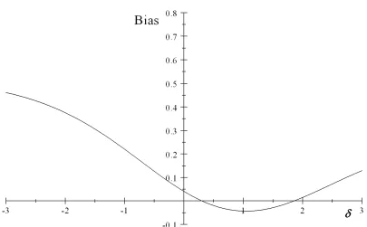
2.1 Plot of bias on magnitude of confoundingδ with 2SPS approach: ρA =
0,ρC = 0.8, ω1C = 0.6,ωC0 = 0.3. . . 32
2.2 Plot of bias on magnitude of confoundingδ with 2SPS approach: ρA =
0,ρC = 0.5, ω1C = 0.6,ωC0 = 0.3. . . 32
2.3 Plot of bias on magnitude of confoundingδ with 2SPS approach: ρA =
0,ρC = 0.5, ω1C = 0.06, ω0C = 0.03. . . 33
2.4 Plot of bias on magnitude of confoundingδ with 2SPS approach: ρA =
0,ρC = 0.5, ω1C = 0.006, ω0C = 0.003. . . 33
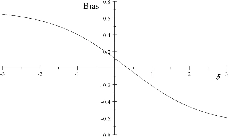
2.5 Plot of bias on magnitude of confoundingδ with 2SRI approach: ρA =
0,ρC = 0.8, ω1C = 0.6,ωC0 = 0.3. . . 34
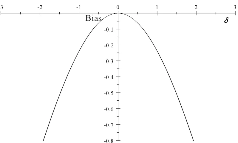
2.6 Plot of bias on magnitude of confoundingδ with 2SRI approach: ρA =
0,ρC = 0.5, ω1C = 0.6,ωC0 = 0.3. . . 34
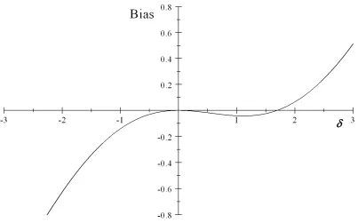
2.7 Plot of bias on magnitude of confoundingδ with 2SRI approach: ρA =
0,ρC = 0.5, ω1C = 0.06, ω0C = 0.03. . . 35
2.8 Plot of bias on magnitude of confoundingδ with 2SRI approach: ρA =
3.1 Comparison of variance between 2SPS and 2SRI with sample size N=500. 66 3.2 Comparison of MSE between 2SPS and 2SRI with sample size N=500. 66 3.3 Comparison of variance between 2SPS and 2SRI with Sample Size
Chapter 1
Introduction
Chapter 2
Bias of Causal Inference for the
Odds Ratio Using Two-Stage
Instrumental Variable Methods
2.1
Introduction
Instrumental variable (IV) methods are used to estimate effects of receiving treat-ment or exposure to risk factor on outcome when there is unmeasured confounding in medical research, such as in clinical trials under non-adherence to treatment (40) or observational studies (41; 42). We present closed form expressions of asymptotic bias for the causal odds ratio from two-stage logistic regressions, which is an extension of the conventional IV method for continuous outcomes to a binary outcome.
associated with treatment; b) it has no direct causal effect on the outcome; and c) it is independent of all (unmeasured) confounders of the treatment-outcome relation-ship (41; 43; 45; 46). Note that in randomized trials, the randomized treatment assignment IV is independent of all confounders because it is randomized. In an observational study, the IV could be associated with measured confounders as long as it is independent of all unmeasured confounders of the treatment-outcome rela-tionship conditional on the measured confounders, and the measured confounders are controlled for in the analysis (45). Under these conditions, IV analysis of the treatment-outcome relationship controls for measured and unmeasured confounding (43; 47; 48; 49).
rate of compliance might differ from the trial (51; 52).
Besides clinical trials, IV methods are used in observational studies, such as data-based evaluations of the effect of medication on clinical or adverse outcomes. IVs such as physician’s prescribing preference (101; 54; 55; 111; 57), clinic or hospital (58),or geographic region (59; 93; 61) have been used to adjust for confounders of the intervention-outcome relationship.
to other sub-groups including anyone who takes the treatment or all patients. The estimands for other types of estimators based on structural mean models can be interpreted similarly (62; 63).
For binary outcomes, the IV approach has been extended in different ways for inference based on odds ratios under logistic models, where the odds ratio is inter-preted as the effect of treatment on outcome in compliers. Those approaches include the Bayesian logistic model estimated with Markov-Chain Monte Carlo techniques (64), the structural mean model (SMM) (65; 66; 67), and a multi-stage approach including an estimation step for the prediction of treatment as a function of the IV (68).
Give the focus of much of the clinical trials literature on the causal effect of treatment in compliers, there is a need for assessment of the 2SPS and 2SRI two-stage logistic estimators with respect to this causal effect. To achieve this goal, we present analytical and simulation results for the bias of these two estimators under a causal logistic model expressed in terms of potential outcomes under the principal stratification framework, following the results of Angrist et al. (43) for the additive model. We also confirm our analytic result with simulations, and the simulations further reveal patterns of bias for different ranges of confoundings. Our bias evaluation is for a different context from that of Terza et al. (39), who focused on the causal odds ratio in the total population conditional on the unmeasured confounder, whereas we focus on the causal odds ratio among compliers.
2.2
Assumption and Notation
re-lationship in observational studies; 3) Exclusion restriction, which means that any effect of treatment assignment on outcomes must be via an effect of treatment assign-ment on treatassign-ment received; 4) Nonzero average causal effect of treatassign-ment assignassign-ment on treatment received, which means that the treatment assignment should be associ-ated with treatment received; and 5) Monotonicity, which means that there is no one who would do the opposite of his/her treatment assignment regardless of the actual assignment.
With the above five assumptions, we first define R and Z as the treatment as-signment and treatment received variables, respectively. First, R=1 denotes that a patient is assigned to the study treatment, and R=0 means a patient is assigned to the other treatment (or non-treatment), thus R is the IV. Similarly, Z=1 means that a patient receives the study treatment, and Z=0 means that a patient receives the other treatment (or non-treatment). Additionally, Y(1) and Y(0) are the variables for potential outcomes. Y(1) indicates what the outcome for a patient would be if this
patient were to take the study treatment, and Y(0) indicates what the outcome for
this patient would be if he/she were to take the other treatment (or non-treatment). In contrast, Y is the observed outcome. Similarly, Z(1) and Z(0) are the variables
for potential treatment. Z(1) indicates what treatment a patient would take if this
patient were assigned to the study treatment, and Z(0) indicates what treatment this patient would take if he/she were assigned to the other treatment (or non-treatment). Based on the principal stratification and potential outcome framework, patients are defined as always-takers (AT) ifZ(1) = 1 and Z(0) = 1; compliers (C) if Z(1) = 1 and
Z(0) = 1.
Accordingly, we define the following parameters in the principal stratification framework:
ωA1 = Pr Y(1) = 1|AT
,
ωC1 = Pr Y(1) = 1|C
,
ωN1 = Pr Y(1) = 1|N T
,
ωA0 = Pr Y(0) = 1|AT
,
ωC0 = Pr Y(0) = 1|C
,
ωN0 = Pr Y(0) = 1|N T
,
r= Pr (R = 1), ρA= Pr(AT), ρC = Pr(C).
With our monotonicity assumption, there are no defiers (43), i.e., P r(DF) = 0. Hence,
Pr(N T) = ρN = 1−ρA−ρC.
The causal log odds ratio for compliers is parameterized as:
ψ =logitPr Y(1) = 1|C
−logitPr Y(0) = 1|C =logit ω1C
−logit ωC0
.
2.3
Bias of Two-Stage Predictor Substitution (2SPS)
In this section, we derive a closed form expression for the probability limit of the two-stage 2SPS logistic regression estimator based on the principal stratification framework and assumptions. We can then obtain closed form expressions for the bias, which is the difference between the expected value of the two-stage regression estimator and the causal log odds ratio.
2.3.1
Probability limit of the estimator
The first stage regression is the treatment received on the treatment assignment R as the IV. Let D=E(Z|R) and ˆD be an estimator of D (e.g., maximum likelihood) such that ˆDconverges in probability toD, ˆD= ˆE(Z|R). Two-stage logistic regression estimates the causal log odds ratio with the coefficient for ˆDin the logistic regression of Y on ˆD. Let ˆξ be an estimator (e.g., maximum likelihood) of the log odds ratio for D in the logistic regression of Y on D, and let ˆξ∗ be the estimator of the log odds ratio for ˆD in the logistic regression of Y on ˆD(i.e., the two-stage 2SPS estimator). As the sample size gets larger, ˆD−→D and|ξˆ∗−ξ|ˆ −→p 0 (74; 75), i.e., ˆξ∗ converges in probability to ξ under the true model conditional on D, which is P(Y = 1|D) =
expit(η+ξD). We now find an expression for ξ as a function of the log odds ratio for treatment received among compliers under the principal stratification framework. When R=0, only takers will receive the treatment; when R=1, both always-takers and compliers will get the treatment. It follows that:
and
d1 =E(Z|R= 1) =ρA+ρC. (2.3.2)
Then for the second stage logistic regression we have:
logitPr (Y = 1|R= 0) =logitPr (Y = 1|D=d0)
=η+ξd0,
logitPr (Y = 1|R= 1) =logitPr (Y = 1|D=d1)
=η+ξd1.
Solving the above two equations for ξ, we have:
ξ= logitPr (Y|R= 1)−logitPr (Y|R= 0)
d1−d0
.
Under the five assumptions stated in Section 2 and the above parameter settings, the probability of observed Y given R can be expressed as the conditional proba-bility of potential outcome Y(0) and Y(1). We can then calculate Pr (Y|R = 1) and
Pr (Y|R= 0) as follows:
logitPr (Y|R= 1) =logit ρAωA1 +ρCω1C+ω
0
N −ρAωN0 −ρCωN0
,
logitPr (Y|R= 0) =logit ρAωA1 +ρCω0C+ω
0
N −ρAωN0 −ρCωN0
The full proof of these equations is in Appendix A1. From the above equation, we can calculate ξ as follows:
ξ = logitPr (Y|R = 1)−logitPr (Y|R= 0)
d1−d0
(2.3.3)
=
logit(ρAωA1 +ρCω1C+ωN0 −ρAωN0 −ρCω0N)− logit(ρAω1A+ρCωC0 +ωN0 −ρAω0N −ρCωN0)
ρC
.
Since ˆξ converges in probability to ξ, equation (2.3.3) is a closed form expression for the probability limit of the two-stage logistic regression estimator of ˆξ.
2.3.2
Bias analysis
Having derived the closed form expression of ξ, we can calculate the difference between ψ and ξ, the asymptotic bias of the two-stage logistic regression.
B2SP S =ξ−ψ (2.3.4)
= 1 ρC
logit(ρAωA0 +ρCω1C+ω0N −ρAωN0 −ρCω0N) −logit(ρAωA0 +ρCω0C+ω0N −ρAωN0 −ρCω0N)
− logit ωC1
−logit ω0C
= 1 ρC
logit(ρAωA0 +ρCω1C+expit(logit(ωC0) +δ)ρN) −logit(ρAωA0 +ρCω0C+expit(logit(ωC0) +δ)ρN)
− logit ωC1−logit ω0C.
In the above equation, we re-parameterize the ω0
N and introduce a new parameter δ
as follow,
then
ωN0 =expit logit ω0C+δ=ωC0 e δ
ω0
Ceδ−ωC0 + 1 .
The parameterδis the difference betweenω0
N andωC0 on the logit scale, so it is the log
odds ratio of never-takers over compliers regarding the outcome. Given differences between principal strata are due to unmeasured confounders related to outcome, δ
in equation (2.3.4) can be interpreted as the magnitude of confounding, where δ = 0 implies no confounding because ω0
N=ω0C.
From the equation (2.3.4), we can easily see:
a) When ρC = 1 (every one is a complier), B2SP S = 0. This is because when ρC = 1, bothρA and ρN are 0. In equation (2.3.4), if we replace ρC by 1 and both ρA
and ρN by 0, we have B2SP S = 0.
b) When ω1
C =ω0C (there is no causal effect), B2SP S = 0. If we replaceωC1 byωC0
in equation (2.3.4), all terms are canceled out and we have B2SP S = 0.
c) The bias function does not include R, thus bias is not related to Pr(R = 1). d) Bias can exist even when there is no confounding, that is, when ρA = 0 and ω0
C =ωN0. Replacing ρA by 0 in equation (2.3.4), we have
B2SP S =
logit(ρAωA1 +ρCω1C+ω0N −ρAωN0 −ρCω0N) −logit(ρAωA1 +ρCω0C+ω0N −ρAωN0 −ρCω0N)
ρC
−logit ωC1+logit ωC0
= logit(ρCω
1
C +ωN0 −ρCωN0)−logit(ωN0) ρC
−logit ωC1+logit ωC0.
In this equation, B2SP S is generally not 0, becauseρC in the denominator can not be
With the closed form expression (2.3.4), we can analyze the magnitude of bias under different parameter settings according to specific scenarios. To simplify the analysis and show the relationship between bias and confounding, we create four such scenarios when there are no always-takers. We plot bias against δ while fixing all other parameters in Fig. 2.1 to 2.4.
All four plots show that the bias is not 0 when there is no confounding (δ = 0). When the compliance rate decreases from 0.8 to 0.5, the bias on the logit scale is about 5 time larger (compare plot 2.1 and plot 2.2). Comparing plot 2.2 and plot 2.3, we can see that when the event rate is lower, the bias range is larger, but when the event rate is decreased from 0.03 to 0.003 (Fig. 2.4), the absolute bias does not increase further.
2.4
Bias of Two-Stage Residual Inclusion (2SRI)
In this section, we extend to the 2SRI estimator, the derivation in Section 3 of bias of the 2SPS under the principal stratification framework. In the first stage regression of treatment received on the treatment assignment R as an IV, the residual is E =Z −E(Z|R), and the second stage regression model is
P r(Y = 1) =expit(λ0+λ1Z+λ2E). (2.4.1)
The estimator ofλ1 is an estimate of the causal log odds ratio for receiving treatment
difference between the probability limit of the estimator ofλ1 and the causal log odds
ratio among compliers.
2.4.1
Closed form expression for the probability limit of the
estimator
For the 2SRI approach, in general, equation (2.4.1) is not the true model for
P r(Y = 1|Z, E), as the true model includes the interaction term between Z and E; this makes it much more difficult to develop a closed form expression for the probabil-ity limit of the estimator. However, if we assume that there are no always-takers, so that Pr (Z = 1, R= 0) = 0, then the true model does not have the interaction term and the 2SRI model in equation (2.4.1) is the true model (see the details in Appendix A2). In this section, we develop a closed form expression for the probability limit of the estimator of λ1 only under the no always-taker assumption. The no always-taker
assumption is true in clinical trials when patients in the placebo group cannot access the study drug. In contrast, the bias results for the 2SPS estimator depend on a true model conditional on just Z (treatment-received) that does not require the absence of always-takers.
The residual E =Z −E(Z|R) is estimated from the first stage regression, and is included as a covariate in the second stage regression. Letting ˆE =Z −Eˆ(Z|R), we consider the second stage regression P r(Y = 1|Z,Eˆ) =expit(λ0+λ1Z +λ2Eˆ). The
2SRI approach estimates the causal log odds ratio with the estimated coefficient for
for Z in the logistic regression of Y on Z and E, and let ˆλ∗1 denote the estimated coefficient for Z in the logistic regression of Y on Z and ˆE. As the sample size gets larger, ˆE −→Eand|λˆ∗1−λˆ1|
p
−→0 (74; 75). The estimator ˆλ∗1converges in probability to λ1 under the model P r(Y = 1|Z, E) = expit(λ0 +λ1Z+λ2E) when there are no
always-takers. When there are always-takers, the 2SRI model is misspecified. In this situation, ˆλ∗1 estimated from the second stage logistic regression converges to the point that minimizes the Kullback-Leibler distance between the family of probability distributions being maximized over the true probability distribution (76).
Under the no always-taker assumption, we can find an expression forλ1 as follows.
From the equations (2.3.1) and (2.3.2), we have
E(Z|R) =ρA+ρCR,
so
E =Z −E(Z|R) = Z−ρA−ρCR.
Note that Z, E and Z, R contain the same information; i.e., knowing Z, E tells us
Z, Rand vice versa, so thatP r(Y = 1|Z, E) =P r(Y = 1|Z, R). For the second stage regression, we have
logitPr (Y = 1|Z, E) (2.4.2) =λ0+λ1Z+λ2E
=λ0+λ1Z+λ2(Z−ρA−ρCR)
=λ0−λ2ρA+ (λ1+λ2)Z−λ2ρCR
Then we have three equations based on the possible values of Z and R ((Z=1,R=0) is not possible because there are no always-takers):
logitPr (Y = 1|Z = 1, R= 1) (2.4.3) =logitPr Y(1) = 1|Z = 1, R= 1
=logit
ρA ρA+ρC
ω1A+ ρC
ρA+ρC ω1C
=λ0−λ2ρA+ (λ1+λ2)−λ2ρC,
logitPr (Y = 1|Z = 0, R= 1) (2.4.4) =logitPr Y(0) = 1|Z = 0, R= 1
=logitPr(Y(0) = 1|N T) =logit(ω0N)
=λ0−λ2ρA−λ2ρC,
logitPr (Y = 1|Z = 0, R = 0) (2.4.5) =logitPr Y(0) = 1|Z = 0, R = 0
=logit
1−ρA−ρC
1−ρA
ω0N + ρC 1−ρA
ωC0
=λ0−λ2ρA.
Solving equations (2.4.3), (2.4.4) and (2.4.5) for λ1 yields the closed form expression
for λ1 as:
λ1 =logit
ρA ρA+ρC
ω0A+ ρC
ρA+ρC ω1C
−logit(ω0N) (2.4.6)
− 1 ρC
logit
1−ρA−ρC
1−ρA
ωN0 + ρC 1−ρA
ωC0
+ 1
ρC
2.4.2
Bias analysis
With the closed form expression for the probability limit of ˆλ1, we can calculate B2SRI, the bias defined as the difference between the log odds ratio for
treatment-received among compliers and the estimated log odds ratio with the 2SRI approach.
B2SRI =λ1−ψ (2.4.7)
=logit
ρA ρA+ρC
ωA1 + ρC
ρA+ρC ωC1
−logit(ωN0)
− 1 ρC
logit
1−ρA−ρC
1−ρA
ω0N + ρC 1−ρA
ωC0
+ 1
ρC
logit(ωN0)
−logit ωC1
+logit ωC0 =logit
ρA ρA+ρC
ωA1 + ρC
ρA+ρC ωC1
−logit expit logit ω0C+δ − 1
ρC logit
1−ρA−ρC
1−ρA
expit logit ωC0 +δ
+ ρC 1−ρA
ω0C
+ 1
ρC
logit expit logit ωC0+δ−logit ωC1+logit ωC0.
δ is the same parameter as in equation (2.3.4). The following conclusions follow from equation (2.4.7):
a) When ρC = 1 (every one is a complier), B2SRI = 0. If ρC = 1, both ρA and ρN
equal to 0. Plug in these values of ρC,ρA and ρN to the equation (2.4.7), B2SRI = 0.
b) When ω0
C = ωN0, and ωA1 = ωC1 (there is no confounding), we replace ωN0 with ω0
C, and ωA1 with ωC1 in equation (2.4.7), yielding B2SRI = 0. That is, when there is
no confounding, the 2SRI approach is unbiased.
As in section 3 with the 2SPS estimator, we use equation (2.4.7) to analyze the magnitude of bias of the 2SRI estimator under different scenarios as in Fig. 2.4-2.8.
the bias of the 2SRI estimator is zero. The first scenario (Fig. 2.5) shows that when the compliance rate is high (0.8), the bias is small for a wide range of confounding. The second scenario (Fig. 2.6) shows that if the outcome is not rare, the bias is very small unless δ is smaller than -1 or greater than 2, which means that the odds ratio comparing compliers to never-takers with respect to the potential outcomes is smaller than 0.37 or greater than 7.4. These scenarios correspond to very strong confounding. Fig. 2.7 shows the scenario when the outcome is rare, with ωC1 and ω0C one tenth of those in scenario 1, The bias for this scenario is larger than that of scenario 1, but the bias is still moderate if the confounding is not very severe. In scenario 4 (Fig. 2.8), we make the outcome even rarer. The magnitude of bias does not change much compared to the bias under scenario 3. Therefore, we can conclude that for the 2SRI model, there is bias when there is confounding, but the bias is small to moderate if the confounding is not severe.
2.5
Simulation
2.5.1
Simulation algorithm
We simulated the data sets according to the following algorithm:
Step 1: Generate a data set with total number of N subjects. Among these subjects, always-takers (ATs), compliers (Cs), and never-takers (NTs) are generated from a multinomial distribution with probability of ρA for ATs, probability of ρC for
step can be implemented by W=t(rmultinom(n, 1, c(ρA,ρC,ρN))).
Step 2: With the probability of P r(R = 1) = r, randomly assign about rN of the subjects to R=1 and the rest of (1−r)N subject to R = 0. This step can be implemented by R=t(rmultinom(n, 1, c(r,1-r))) in the package R.
Step 3: Simulate Y(0) and Y(1) based on the value of AT, C or NT, and the parameter ω1
A, ωC1, ωN1 , ω0A, ωC0, and ω0N. For instance, if an subject is AT, then P r(Y(0) = 1) = ω0A, and P r(Y(1) = 1) = ωA1. With these probabilities, we can createY(1) and Y(0) with the binomial distribution. We implemented this step in the package R with the following program:
prY0=W[,1]*ω0A+W[,2]*ω0C+W[,3]*ωN0
dim(prY0)=c(n,1) prY1=W[,1]*ω1
A+W[,2]*ω1C+W[,3]*ωN1
dim(prY1)=c(n,1)
Y0=apply(prY0, 1, function (x) rbinom(1,1,x)) Y1=apply(prY1, 1, function (x) rbinom(1,1,x))
Step 4: Based on AT, C or NT, and R, determine Z. For instance, if an observation is in either the AT or C group, and the treatment assignment R=1, then Z=1.
2.5.2
Simulation results
For each setting, we ran the simulation 2000 times, with the sample size of n=10,000. For both 2SPS and 2SRI approaches, we simulated data with different selection of parameters. As examples, Table 2.1 shows the results with the parameter settings without always-takers: ρA = 0; ρC = 0.5 (thus ρN = 0.5); ω0C = 0.3 or ωC0 = 0.03; ω1C = 0.6 or ωC1 = 0.06; δ varies among 2, 1.5, 1, 0.5, 0, -0.5, -1, -1.5 or -2. For these simulations, the bias is calculated as the difference between the mean of estimated log odds ratio ( ˆξ for 2SPS and ˆλ1 for 2SRI) and the log odds ratio among
compliers ψ. The mean square of error (MSE) is calculated as the mean square of the difference between the estimated log odds ratio and the log odds ratio among compliers.
Under all parameter settings without always-takers, the bias resulting from simu-lations is consistent with the analytic results, and when there is no confounding, the bias is not zero for 2SPS but is zero for 2SRI (Table 2.1). The simulation results of MSE follow the same pattern as the results for absolute bias with these large sample simulations. We are currently doing further research on the MSE properties of the different estimators.
We also performed simulations including always-takers with the parameter settings:
simulated data is consistent with the analytic results for the 2SPS approach when there are always-takers. For 2SRI, the results show that the bias is smaller than for 2SPS, and is close to 0 when δ is 0, but for some parameter settings with strong confounding, the bias is larger than for 2SPS.
2.6
Discussion
An important contribution of this research is the expression of the conditional distribution of observed outcomes Y given treatment assignment R as a function of the probability of compliance and the conditional distribution of potential outcomes
Y(0) and Y(0), given compliance status. With this contribution, we can analytically
present probability limits and therefore the bias of the estimators of the causal effects of treatment given compliance and treatment status. Further, we provide analytic estimates of bias for a variety of situations. These analytic estimates of bias can help researchers evaluate if the bias is small under specific conditions (e.g. high compliance, and moderate confounding). Hence, our results can be used as a guide for deciding if the 2SRI or 2SPS strategy is appropriate. This method can be potentially applied to the bias analysis of causal inference with other non-linear two-stage regressions, such as regressions of probit models and log linear models.
When the 2SRI or 2SPS is appropriately used, these approaches have the ad-vantage that they are very easy to implement with any software package that can do logistic regression (e.g., SAS, R, or STATA). Logistic regression is used for both the first and second stages of either the 2SRI or 2SPS procedures. The predicted or residual values from the first stage logistic regression of treatment on the IV are used as covariates in the second stage logistic regression: the predicted value of treat-ment replaces observed treattreat-ment for 2SPS, whereas the residual from the first stage regression is added as a covariate along with observed treatment for 2SRI.
δ
Fig 2.1. Plot of bias on magnitude of confounding δ with 2SPS approach:
ρ
A=0, ρC=0.8,ω1c=0.6, ω
0
c =0.3.
δ
Fig 2.2. Plot of bias on magnitude of confounding δ with 2SPS approach:
ρ
A=0, ρC=0.5,δ
Fig 2.3. Plot of bias on magnitude of confounding δ with 2SPS approach: ω₁=0, ω₂=0.5,
ω₁₂=0.06, ω₀₂=0.03.
δ
Fig 2.4. Plot of bias on magnitude of confounding δ with 2SPS approach:
ρ
A=0, ρC=0.5,ω1
δ
Fig 2.5. Plot of bias on magnitude of confounding δ with 2SRI approach:
ρ
A=0, ρC=0.8,ω1c=0.6, ω
0
c =0.3.
δ
Fig 2.6. Plot of bias on magnitude of confounding δ with 2SRI approach:
ρ
A=0, ρC=0.5,δ
Fig 2.7. Plot of bias on magnitude of confounding δ with 2SRI approach:
ρ
A=0, ρC=0.5,ω1c=0.06, ω
0
c =0.03.
δ
Fig 2.8. Plot of bias on magnitude of confounding δ with 2SRI approach:
ρ
A=0, ρC=0.5,ω1c=0.006, ω
0
Table 2.1. Comparison of simulation results and analytic results when there are no always-takers.
2SPS 2SRI
ω0
C ω1C
True
LogOR δ Regression LogOR by Observed Bias
Analytic Result
of Bias MSE Regression LogOR by Observed Bias
Analytic Result
of Bias MSE
0.3 0.60 1.2528 -2.0 1.6295 0.3768 0.3754 0.1500 0.6256 -0.6272 -0.6266 0.4095
-1.5 1.5601 0.3073 0.3061 0.1024 0.9112 -0.3416 -0.3415 0.1295
-1.0 1.4740 0.2213 0.2200 0.0567 1.1127 -0.1400 -0.1410 0.0301
-0.5 1.3813 0.1286 0.1263 0.0238 1.2244 -0.0284 -0.0309 0.0095
0.0 1.2961 0.0433 0.0405 0.0088 1.2559 0.0031 0.0000 0.0075
0.5 1.2362 -0.0166 -0.0200 0.0069 1.2383 -0.0145 -0.0179 0.0071 1.0 1.2079 -0.0449 -0.0435 0.0090 1.2103 -0.0425 -0.0413 0.0088 1.5 1.2228 -0.0300 -0.0289 0.0081 1.2268 -0.0259 -0.0250 0.0079
2.0 1.2666 0.0138 0.0145 0.0080 1.3172 0.0644 0.0651 0.0123
0.03 0.0600 0.7246 -2.0 1.2894 0.5648 0.5666 0.3901 -0.1732 -0.8978 -0.8474 0.9745
-1.5 1.2215 0.4969 0.4973 0.3131 0.2011 -0.5235 -0.5015 0.3865
-1.0 1.1225 0.3980 0.3994 0.2181 0.4788 -0.2458 -0.2314 0.1432
-0.5 0.9900 0.2654 0.2709 0.1232 0.6522 -0.0724 -0.0589 0.0666
0.0 0.8374 0.1128 0.1175 0.0585 0.7161 -0.0084 0.0000 0.0485 0.5 0.6770 -0.0475 -0.0459 0.0387 0.6630 -0.0616 -0.0571 0.0406 1.0 0.5198 -0.2048 -0.2005 0.0705 0.5002 -0.2243 -0.2169 0.0790 1.5 0.3911 -0.3334 -0.3310 0.1335 0.2658 -0.4587 -0.4525 0.2339
2.0 0.2932 -0.4314 -0.4306 0.2026 -0.0107 -0.7352 -0.7297 0.5593
Table 2.2. Comparison of simulation results and analytic results when there are always-takers.
2SPS 2SRI
ω0
C ω1C
True
LogOR δ Regression LogOR by Observed Bias
Analytic Result
of Bias MSE Regression LogOR by Observed Bias
Analytic Result
of Bias MSE
0.3 0.60 1.2528 -2.0 1.3159 0.0631 0.0615 0.0098 1.2554 0.0026 NA 0.0090
-1.5 1.3007 0.0480 0.0461 0.0081 1.2624 0.0096 NA 0.0085
-1.0 1.2809 0.0281 0.0257 0.0065 1.2677 0.0149 NA 0.0079
-0.5 1.2574 0.0046 0.0016 0.0057 1.2668 0.0140 NA 0.0074
0.0 1.2338 -0.0190 -0.0220 0.0061 1.2559 0.0031 NA 0.0066
0.5 1.2167 -0.0361 -0.0389 0.0073 1.2380 -0.0148 NA 0.0067
1.0 1.2112 -0.0416 -0.0434 0.0083 1.2221 -0.0306 NA 0.0077
1.5 1.2201 -0.0327 -0.0346 0.0077 1.2216 -0.0311 NA 0.0076
2.0 1.2393 -0.0135 -0.0162 0.0071 1.2410 -0.0118 NA 0.0071
0.03 0.0600 0.7246 -2.0 0.8826 0.1580 0.1583 0.0753 0.9577 0.2331 NA 0.1092
-1.5 0.8623 0.1378 0.1390 0.0677 0.9177 0.1931 NA 0.0895
-1.0 0.8312 0.1067 0.1093 0.0578 0.8633 0.1387 NA 0.0677
-0.5 0.7880 0.0634 0.0652 0.0483 0.7983 0.0737 NA 0.0507
0.0 0.7276 0.0030 0.0034 0.0410 0.7250 0.0005 NA 0.0413
0.5 0.6471 -0.0774 -0.0766 0.0421 0.6443 -0.0803 NA 0.0427
1.0 0.5549 -0.1696 -0.1704 0.0598 0.5541 -0.1705 NA 0.0600
1.5 0.4575 -0.2671 -0.2683 0.0971 0.4389 -0.2857 NA 0.1073
2.0 0.3686 -0.3560 -0.3586 0.1472 0.2962 -0.4284 NA 0.2042
2.7
Appendix
A1. Prove that the probability of observed Y given R can be expressed by the following equations.
Pr (Y|R= 1) =ρAωA0 +ρCω1C+ω
0
N −ρAωN0 −ρCωN0,
and
Pr (Y|R= 0) =ρAωA0 +ρCω0C+ωN0 −ρAωN0 −ρCωN0.
In these equations, AT means always-taker, C means complier, and NT means never-taker, and
ω1A= Pr Y(1) = 1|AT
,
ωC1 = Pr Y(1) = 1|C
,
ωN1 = Pr Y(1) = 1|N T
,
ω0A= Pr Y(0) = 1|AT
,
ωC0 = Pr Y(0) = 1|C
,
ωN0 = Pr Y(0) = 1|N T
,
Proof:
Pr Y(1) = 1|Z = 1, R= 1
= Pr Y(1)= 1, Z = 1, R = 1/Pr(R= 1, Z = 1) = Pr(Y
(1) = 1, AT, R= 1) + Pr(Y(1) = 1, C, R= 1)
Pr(R = 1, AT) + Pr(R= 1, C) = Pr(Y
(1) = 1, AT) Pr(R = 1) + Pr(Y(1)= 1, C) Pr(R = 1)
Pr(R = 1) Pr(AT) + Pr(R = 1) Pr(C) = Pr(Y
(1) = 1|AT) Pr(AT) + Pr(Y(1) = 1|C) Pr(C)
Pr(R = 1) Pr(AT) + Pr(R= 1) Pr(C) = Pr(AT)
Pr(AT) + Pr(C)Pr(Y
(1)
= 1|AT) + Pr(C)
Pr(AT) + Pr(C)Pr(Y
(1)
= 1|C) = ρA
ρA+ρC
ω1A+ ρC
ρA+ρC ω1C.
Note: According to the assumptions of the IV, R is independent of Y(1) and the
principal stratum, thus in the above equation, P r(Y(1) = 1, AT, R= 1) =P r(Y(1) =
1, AT)P r(R = 1) and P r(Y(1) = 1, C, R= 1) =P r(Y(1) = 1, C)P r(R = 1). Pr Y(0) = 1|Z = 0, R= 0
= Pr(N T)
Pr(N T) + Pr(C)Pr(Y
(0) = 1|N T) + Pr(C)
Pr(N T) + Pr(C)Pr(Y
(0) = 1|C)
= 1−ρA−ρC 1−ρA
ωN0 + ρC 1−ρA
Pr (Y = 1|R = 1)
= Pr Y(1) = 1, Z = 1|R = 1+ Pr Y(0) = 1, Z = 0|R= 1 = Pr(Y(1) = 1|Z = 1, R= 1) Pr(Z = 1|R= 1)+
Pr(Y(0) = 1|Z = 0, R = 1) Pr(Z = 0|R = 1) =
ρA ρA+ρC
ωA0 + ρC
ρA+ρC ωC1
(ρA+ρC) +ωN0 (1−ρA−ρC)
=ρAωA0 +ρCω1C+ω
0
N −ρAωN0 −ρCωN0,
Pr (Y = 1|R = 0)
= Pr Y(1) = 1, Z = 1|R= 0+ Pr Y(0) = 1, Z = 0|R= 0 = Pr(Y(1) = 1|Z = 1, R= 0) Pr(Z = 1|R= 0)+
Pr(Y(0) = 1|Z = 0, R= 0) Pr(Z = 0|R= 0) =ω0AρA+
1−ρA−ρC
1−ρA
ωN0 + ρC 1−ρA
ω0C
(1−ρA)
=ρAωA0 +ρCω0C+ω
0
N −ρAωN0 −ρCω0N.
A2. Prove: Pr(Y = 1|Z, E) = expit(λ0+λ1Z +λ2E) is not the true model and
Proof: The true model is
Pr (Y = 1|Z, E) = Pr (Y = 1|Z, R) = E(Y|Z, R)
= I(Z=0,R=0)E(Y|Z = 0, R= 0) +I(Z=1,R=0)E(Y|Z = 1, R= 0)
+I(Z=0,R=1)E(Y|Z = 0, R = 1) +I(Z=1,R=1)E(Y|Z = 1, R= 1)
= E(Y|Z = 0, R = 0)
+Z[E(Y|Z = 1, R = 0)−E(Y|Z = 0, R = 0)] +R[E(Y|Z = 0, R = 1)−E(Y|Z = 0, R= 0)] +ZR
E(Y|Z = 1, R= 1)−E(Y|Z = 1, R = 0)
−E(Y|Z = 0, R = 1) +E(Y|Z = 0, R= 0) = λ0+λ1Z+λ2R+λ3ZR.
In the above equations,
λ0 = E(Y|Z = 0, R= 0),
λ1 = [E(Y|Z = 1, R = 0)−E(Y|Z = 0, R= 0)], λ2 = [E(Y|Z = 0, R = 1)−E(Y|Z = 0, R= 0)], λ3 =
E(Y|Z = 1, R= 1)−E(Y|Z = 1, R= 0)
−E(Y|Z = 0, R= 1) +E(Y|Z = 0, R= 0) = E(Y|Z = 1, R= 1)−(λ0+λ1+λ2).
So the true model includes the interaction between Z and R.
becomes
Pr (Y = 1|Z, E) = Pr (Y = 1|Z, R) =E(Y|Z, R)
=I(Z=0,R=0)E(Y|Z = 0, R= 0)
+I(Z=0,R=1)E(Y|Z = 0, R= 1) +I(Z=1,R=1)E(Y|Z = 1, R = 1)
=E(Y|Z = 0, R = 0)
+R[E(Y|Z = 0, R= 1)−E(Y|Z = 0, R= 0)] +Z[E(Y|Z = 1, R= 1)−E(Y|Z = 0, R= 1)] =λ0+λ1R+λ2Z.
In the above equations,
λ0 = E(Y|Z = 0, R= 0),
λ1 = [E(Y|Z = 0, R = 1)−E(Y|Z = 0, R= 0)], λ2 = [E(Y|Z = 1, R = 1)−E(Y|Z = 0, R= 1)].
The true model does not include the interaction term. A3. Some details about the bias analysis.
The bias of 2SPS estimator is:
B2SP S =
logit(ρAωA1 +ρCω1C+ωN0 −ρAωN0 −ρCω0N) −logit(ρAωA1 +ρCω0C+ω0N −ρAωN0 −ρCω0N)
ρC
−logit ωC1+logit ω0C.
One no-confounding scenario is that there are no always-takers, and compliers and never-takers have the same probability of potential outcome, e.g., ρA = 0 and ωC0 = ωN0. Plugging in these values to the above equation, we have,
B2SP S =
logit(0ωA1 +ρCω1C+ω
0
C −0ω
0
C −ρCωC0) −logit(0ω1
A+ρCω0C+ωC0 −0ωC0 −ρCωC0) ρC
−logit ω1C+logit ω0C
= logit(ρCω
1
C+ωC0 −ρCωC0)−logit(ω0C) ρC
−logit ω1C+logit ω0C.
This equation generally not 0. We can easily see that it is 0 if on linear scale instead of logit scale.
b)When there is no confounding, the treatment effect estimated with 2SRI is unbiased.
The bias of the 2SRI estimator with no always-takers is:
B2SRI =λ1−ψ
=logit
ρA ρA+ρC
ω1A+ ρC
ρA+ρC ω1C
−logit(ω0N)
− 1 ρC
logit
1−ρA−ρC
1−ρA
ωN0 + ρC 1−ρA
ω0C
+ 1
ρC
logit(ω0N)
. Plug inρA = 0 andωC0 =ωN0 to this equation, we have: B2SRI =λ1−ψ
=logit
0 0 +ρC
ωA1 + ρC 0 +ρC
ω1C
−logit(ω0C)
− 1 ρC
logit
1−0−ρC
1−0 ω
0
C+ ρC
1−0ω
0
C
+ 1
ρC
logit(ωC0)
−logit ωC1+logit ωC0
=logit ω1C−logit(ω0C)− 1 ρC
logit(ωC0) + 1
ρC
logit(ωC0)
−logit ωC1+logit ωC0
= 0.
Chapter 3
Variance Estimate of Causal Odds
Ratio with Instrumental Variable
Two-Stage Logistic Regression
3.1
Introduction
different two-stage instrumental variable estimators. The two stage logistic regression approaches we consider are the two-stage predictor substitution (2SPS) and two-stage residual inclusion (2SRI) methods (70; 85; 39; 79). We evaluate the bias of these vari-ance estimators relative to the true variability of the IV point estimates by simulations and evaluate the coverage of confidence interval calculated with the variance estima-tor we proposed. In this paper, we use ”treatment” to represent either treatment received or exposure to a risk factor. An IV has the following properties: a) it is associated with treatment; b) it has no direct causal effect on the outcome; and c) it is independent of all unmeasured confounders of the treatment-outcome relationship (45; 40; 41; 86). Under these conditions, the IV analysis of the treatment-outcome relationship controls for measured and unmeasured confounding (43; 47; 48; 49). For randomized trials, the IV is randomized treatment assignment, but for observational studies it needs to be a carefully selected under the above assumptions The 2SPS and 2SRI IV approaches generally involve, as a first stage, the modeling of treatment as a function of the IV and any baseline covariates and then the second stage mod-eling of outcome as some function of predicted treatment and the covariates from the first stage regression. Under the 2SPS approach, predicted treatment from the first stage model replaces observed treatment as the principal covariate in the sec-ond stage model relating outcome to treatment (88; 55). Under the 2SRI method (70; 85), predicted and observed treatment are used to compute a residual that is included as a covariate in the second stage model where the principal covariate is observed treatment.
the general instrumental variable strategy (43). Under the potential outcome frame-work, they set up principal stratification framework under the assumptions that the proposed IV is associated with treatment, is independent of unmeasured confounders given the measured confounders and that the IV only affects outcome through treat-ment received and there are no defiers. With the principal stratification framework, patients are classified by the compliance status of treatment assignment as always-takers, compliers and never-takers. For the linear model, they analytically proved that under the above assumptions, the treatment effect estimated by the 2SPS IV method can be interpreted as average causal effect of compliers, which is called local average treatment effect (LATE), or compliers average causal effect (CACE). Since the 2SPS and 2SRI approaches give the same estimates with linear regression (70), the linear 2SRI also has the interpretation of LATE or CACE (43; 85).
For the linear two stage methods, the naive variance estimate obtained with ordi-nary least squares under the second stage regression model of treatment on outcome is not correct, since it does not adjust for the variability of the predicted treatment as a covariate in this model. The variance estimator for the 2SPS IV estimator is based on a heteroskedasticity-robust or sandwich estimator of variance involving cross products of the predicted treatment vector and a scalar dispersion factor based on the observed treatment factor (75). For the 2SRI approach, we have not found any published research on the variance estimator, but the estimate needs to be adjusted in a similar way, as the 2SRI and 2SPS approaches yield the same estimate of treatment effect for the linear case (70).
3.2
Notation and parameter setting
We define R as the IV, which in randomized trial setting is randomized treatment assignment, and Z as the treatment received. R=1 means that a patient is assigned to the study treatment, and R=0 means a patient is assigned to the other treatment (or no treatment). Similarly, Z=1 means that a patient receives the study treatment, and Z=0 means that a patient receives the other treatment (or non-treatment). Y is the observed binary outcome. With this definition, R is the instrumental variable. Under the principal stratification framework which provides the causal estimand for the two stage procedures, we also define as the probability of a subject being in the always-taker (AT) class, and as the corresponding probability for the complier class. Under the principal stratification framework with the no-defier assumption, only ATs can get the study treatment when they are assigned to other treatment or no treatment. Consequently, the first stage logistic regression for both the 2SPS and 2SRI approaches is parameterized as:
E(Z|r) =expit rTρ
=expit(ρA+ρCr). (3.2.1)
In the above equation, rT = (1, r) and ρT = (ρ A, ρC).
For the 2SPS approach, the second stage logistic regression is the outcome on the predicted treatment-received (i.e., the expected value of Z conditional on R) from the first stage regression, which is,
treatment effect isλ2.
For the 2SRI, the second stage logistic regression is the model of outcome on treatment received AND the residual from the first stage regression:
EY = expit(λ1+λ2zi+λ2ˆe) (3.2.3)
= expit(λ1+λ2zi+λ2[zi−expit(ρA+ρCri)]).
With this regression, the treatment effect is also λ2. Our goal is to derive and
evaluate variance estimators for the 2SPS and 2SRI estimators of λ2.
3.3
Variance estimate of 2 stage logistic regression
We use the Wooldridge’s approach for two-step M estimation to derive the variance estimator of the 2SPS and 2SRI estimators of the CACE log odds ratio for receiving treatment. Accordingly, we derive separate objective functions for the first and second stage models from which we obtain separate score and Hessian equations.
3.3.1
Variance estimate of 2SPS
For the 2SPS approach, we derive score and Hessian functions for the first and second stage models. For the first stage model in (3.2.1), the objective function for the parameters is defined as the log of the binomial mass function for an individual response:
The estimators of ρA and ρC maximize Pq1(z,r;ρ), and solves the first-order
con-dition:
X
si(z,r;ρ) = 0, (3.3.2)
where si(z,r;ρ) is the two-dimensonal vector score for the objective function q1(z,r;ρ) for an individual subject, derived by taking the first order partial
deriva-tives of q1(z,r;ρ) with respect to the dimensional parameter vectorρ.
Similarly, let denote the Hession matrix ofq1(z,r;ρ) with respect toρfor an
indi-vidual subject asH1(z,r;ρ)≡∂2q1(z,r;ρ)/ ∂ρ∂ρ0, then by a Taylor series expansion
with ˆρ converging in probability to ρ∗, we have, ˆ
ρ−ρ∗ ≈XH1(z,r; ˆρ)
−1
−Xs1(z,r; ˆρ)
, (3.3.3) where ˆρT = ( ˆρA,ρˆC) from the first stage regression.
For the second stage of the 2SPS approach, with ρreplaced with ˆρ from the first stage, the objective function based on equation (3.2.2) is,
q2(y,r; ˆρ, λ) = yˆzTλ−ln 1 + exp ˆzTλ
(3.3.4) = y(λ1+λ2zˆ)−ln [1 + exp (λ1+λ2zˆ)]
= y(λ1+λ2expit( ˆρA+ ˆρCr))−ln [1 + exp (λ1+λ2expit( ˆρA+ ˆρCr))].
The estimators of λ1 and λ2 maximize q2(y,r; ˆρ, λ) , i.e., solves the first-order
condition,
X
s2(yi,ri; ˆρ,λ) = 0, (3.3.5)
where s2(yi,ri; ˆρ, λ) is the score of the objective function q2(y,r; ˆρ,λ) for
the objective function q2(y,r; ˆρ, λ), with respect to λ.
We then take the following Taylor expansion with ˆλ converging in probability to
λ∗, we have, ˆ
λ−λ∗ ≈XH2
yi,ri; ˆρ,λˆ
−1
−Xs2
yi,ri; ˆρ,λˆ
, (3.3.6) where s2
yi,ri; ˆρ,ˆλ
and H2
yi,ri; ˆρ,λˆ
are obtained from s2(yi,ri; ˆρ, λ) and H2(yi,ri; ˆρ, λ) respectively by replacing λ with ˆλ. Given the series expansion in
(3.3.6), one variance estimate of bλ is, b
Vλˆ
naive =
X
H2
yi,ri; ˆρ,λˆ
−1X
s2
yi,ri; ˆρ,λˆ
s2
yi,ri; ˆρ,λˆ
T X
H2
yi,ri; ˆρ,ˆλ
−1
. (3.3.7)
However, this variance estimate does not take into account that the variability of ˆ
z through ˆρ. That is, it does not take into account the series expansion in (6) for ˆ
ρ. Consequently, we achieve such an adjustment by incorporating the Taylor series expansion in (3.3.3) with the following Taylor series expansion of P
s2(yi,ri; ˆρ,λ)
around ρ∗, the probability limit of ˆρ, as follows: X
s2(y,r; ˆρ, λ)≈
X
s2(y,r;ρ∗,λ) +
X∂s2(y,r;ρ∗, λ)
∂ρ (ˆρ−ρ
∗
), (3.3.8) where ∂s2(y,∂rρ;ρ∗,λ) is the partial derivative of s2(y,r;ρ∗,λ) with respect to ρ
eval-uated atρ∗. From the approximation in (3.3.3) for (ˆρ−ρ∗), the expansion in (3.3.3) is asymptotically equivalent to:
X
s2(y,r; ˆρ,λ) ≈
X
s2(y,r;ρ∗,λ) +
X∂s2(y,r;ρ∗, λ)
∂ρ
X
H1(z,r; ˆρ)
−1
−Xs1(z,r; ˆρ)
Based on (3.3.9), we follow the general case of Wooldridge (75) by adjusting the score evaluated at ˆρ and ˆλ , s2
y,r; ˆρ,λˆ, as gy,r; ˆρ,λˆ,
gy,r; ˆρ,λˆ=s2
y,r; ˆρ,λˆ+X
∂s2
y,r; ˆρ,λˆ
∂ρ
X
H1(zi,ri; ˆρ)
−1
(−s1(zi,ri; ˆρ)).
(3.3.10) Replacing the s2
yi,ri; ˆρ,λˆ
by gyi,ri; ˆρ,λˆ
, the variance estimator for the 2SPS estimator of λ, adjusted for the first stage regression estimate of ρis,
b V ˆ λ adjust = X H2
yi,ri; ˆρ,λˆ
−1X
g
yi,ri; ˆρ,λˆ
g
yi,ri; ˆρ,λˆ
T
X
H2
yi,ri; ˆρ,λˆ
−1
. (3.3.11)
3.3.2
Variance estimator for the 2SRI approach
For the 2SRI approach, we take the same strategy as above and adjust the second stage objective function forλwith the corresponding approximation in (3.3.3) to ad-just forhatρunder the first stage regression. Accordingly, the second stage objective function for λunder the 2SRI approach is:
q2(y, z; ˆe,λ) = y(λ1+λ2z+λ3eˆ)−ln(1 +exp(λ1+λ2z+λ3eˆ)) (3.3.12)
The corresponding adjusted score is,
g
y, z; ˆe,λˆ
=s2
y, z; ˆe,λˆ
+X
∂s2
y, z; ˆe,λˆ
∂ρ
X
H1(zi,ri; ˆρ)
−1
(−s1(zi,ri; ˆρ))
For two stage linear regression, we analytically prove that the above 2SPS and 2SRI variance estimators, which are equivalent, equal the heteroskedasticity-robust variance estimate of the simple two stage linear regression (See the detail in attach-ment A).
3.4
Simulations
Since our research is focused on the causal inference of two stage logistic regression, we simulated data with the principal stratification settings of the Angrist-Rubin model of causal inference. The data sets were generated with the following algorithm.
Step 1: Generate a data set with total number of N subjects. Among these subjects, always-takers (ATs), compliers (Cs), and never-takers (NTs) are generated from multinomial distributions with probability ρA for ATs, ρC for Cs, and ρN for
NTs.
Step 2: With the probability of r, randomly assign rN subjects to R=1 and the rest of (1−r)N subjects to R=0.
Step 3: Create the potential outcomeY(0)andY(1)based on the compliance status
of each subject, and the probability of potential outcome for each compliance status. Step 4: Determine treatment received Z of each subject based on the treatment assignment R and compliance status.
Step 5: With the following equation, determine observed outcome of each subject based on the potential outcome and treatment received,
We simulated data sets with different compliance rates, different confounding fac-tors, and different sample sizes with information from our example data analysis. For each setting of the parameters, we simulated 2000 data sets and performed the 2SPS and 2SRI methods for logistic regression. For each of these estimation approaches, we calculated the simulation-based variance of the log odds ratio estimates, in addi-tion to the averages of the naive variance, adjusted variance, and bootstrap variance estimated at each iteration for the corresponding estimator of the log odds ratio for treatment on outcome. We also used these different variance estimates to calculate 95% coverage estimates for the log odds ratio. Finally, we calculated the mean square error for the 2SPS and 2SRI estimates of the log odds ratio for treatment on outcome.
3.5
Result
the 2SRI approach compared to the 2SPS approach. When the sample size is 5000 (Table 3.2), the variance of both log odds ratio estimators is small, so the MSE is mainly determined by the bias. As shown in Cai et al. (79), both the 2SPS and 2SRI approaches are similarly biased for the log odds ratio of receiving treatment among compliers. In this situation, the MSE of 2SRI approach is close to the 2SPS approach.
3.6
Discussion
In this paper, we applied the theory of two-step M estimation to obtain the ad-justed variance estimators for the 2SPS and 2SRI IV estimators of the log odds ratio of receiving treatment among compliers. Our simulation results show that the ad-justed variance estimators provide good estimates of the simulated variance of the causal log odds ratio. In addition, these adjusted variance estimators perform better than the corresponding bootstrap estimators. We found that the average bootstrap variance is not accurate when the compliance rate is low, which is consistent with other studies that have shown that the validity of bootstrap is questionable when the IV is weakly correlated with the endogenous explanatory variable (92).
Table 3.1. Comparison of adjusted variance estimates with naïve estimates and the variance estimated by bootstrap for the percentage difference from the sample variance of simulation: 2SPS approach with small sample size.
Compliance Rate C
ρ Delta Variance Sample Naïve Estimate (% Difference) Adjusted Variance (% Difference) Bootstrap Estimate (% Difference)
0.3 -3 0.3821 32.85 4.02 12.76
-2.5 0.3839 29.96 3.06 11.37
-2 0.3939 23.52 -0.19 10.78
-1.5 0.3814 23.06 1.95 9.61
-1 0.3717 20.45 3.41 7.22
-0.5 0.3563 19.09 6.65 8.20
0 0.3663 10.11 3.92 9.63
0.5 0.3865 0.98 0.92 8.29
1 0.4108 -5.31 -0.18 7.00
1.5 0.4596 -12.93 -2.48 12.57
2 0.5114 -17.67 -2.37 14.97
2.5 0.5830 -23.37 -4.16 17.15
3 0.6357 -25.73 -3.27 18.43
0.5 -3 0.1206 23.01 2.77 5.79
-2.5 0.1205 22.37 2.84 5.03
-2 0.1223 19.52 1.42 4.72
-1.5 0.1227 17.52 1.20 6.97
-1 0.1240 14.30 0.47 5.15
-0.5 0.1267 9.45 -1.02 5.09
0 0.1254 8.33 1.41 5.50
0.5 0.1250 7.06 4.31 7.04
1 0.1339 -0.49 1.18 5.50
1.5 0.1396 -3.73 1.90 4.83
2 0.1471 -7.15 1.79 8.61
2.5 0.1529 -8.92 2.67 10.06
3 0.1599 -11.40 2.01 8.95
0.7 -3 0.0629 11.81 2.32 2.96
-2.5 0.0628 11.88 2.56 3.26
-2 0.0630 11.38 2.44 3.14
-1.5 0.0637 10.02 1.68 4.32
-1 0.0645 8.34 0.86 3.29
-0.5 0.0657 5.96 -0.34 3.44
0 0.0652 6.33 1.36 2.46
0.5 0.0650 6.24 2.95 2.52
1 0.0688 0.29 -1.07 0.69
1.5 0.0695 -0.83 -0.53 2.13
2 0.0703 -1.85 -0.13 3.48
2.5 0.0708 -2.48 0.31 3.17
3 0.0717 -3.65 -0.13 2.35
Note: Number of iteration of bootstrap p=500; Sample size N=500, Simulation time M=2000. Outcome rate for treatment group ω11= ω 12= ω 13=0.6;
Table 3.2. Comparison adjusted variance estimates with naïve estimates and the variance estimated by bootstrap for the percentage difference from the sample variance of simulation: 2SPS approach with large sample size.
Compliance Rate C
ρ δ Variance Sample Naïve Estimate (% Difference) Adjusted Variance (% Difference) Bootstrap Estimate (% Difference)
0.3 -3 0.1859 30.15 0.64 3.69
-2.5 0.1799 32.28 3.50 3.74
-2 0.1774 30.80 4.24 4.43
-1.5 0.1790 25.12 2.45 6.44
-1 0.1781 20.07 1.87 3.33
-0.5 0.1782 13.81 0.88 4.03
0 0.1798 7.34 0.03 4.44
0.5 0.1838 1.62 -0.09 5.11
1 0.1843 0.98 4.67 7.14
1.5 0.2084 -8.18 0.45 5.57
2 0.2342 -14.09 -1.15 4.10
2.5 0.2614 -18.42 -1.85 5.67
3 0.2892 -22.14 -2.79 5.87
0.5 -3 0.0636 15.97 -3.34 2.66
-2.5 0.0640 14.49 -3.99 1.64
-2 0.0633 14.70 -2.90 0.25
-1.5 0.0628 14.19 -1.94 -0.13
-1 0.0648 8.78 -4.63 0.23
-0.5 0.0653 5.68 -4.71 0.64
0 0.0670 0.96 -5.74 0.81
0.5 0.0675 -1.40 -4.22 1.33
1 0.0687 -3.44 -2.19 0.86
1.5 0.0744 -10.16 -5.27 -1.22
2 0.0800 -15.11 -7.34 -1.94
2.5 0.0833 -16.87 -6.65 0.18
3 0.0860 -18.12 -6.09 0.61
0.7 -3 0.0332 5.86 -3.27 -0.48
-2.5 0.0334 5.13 -3.74 -0.39
-2 0.0331 5.87 -2.76 -0.22
-1.5 0.0332 5.25 -2.85 0.01
-1 0.0336 3.87 -3.43 0.78
-0.5 0.0337 3.11 -3.14 1.73
0 0.0345 0.27 -4.53 2.99
0.5 0.0346 -0.16 -3.38 2.91
1 0.0357 -3.54 -4.98 -1.38
1.5 0.0365 -5.70 -5.54 -1.18
2 0.0370 -6.85 -5.35 -1.43
2.5 0.0374 -7.89 -5.34 -1.39
3 0.0378 -8.54 -5.27 -0.09
Note: Number of iteration of bootstrap p=700. Sample size N=1000, Simulation time M=2000.
Outcome rate for treatment group ω 11= ω 12= ω 13=0.6;
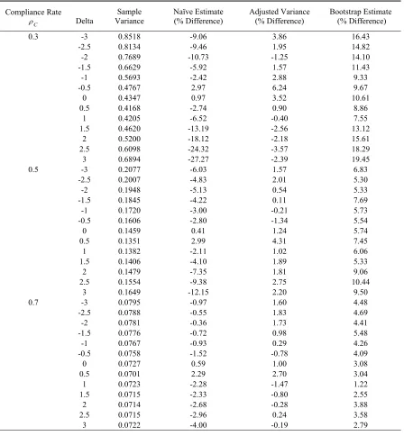
Table 3.3. Comparison of adjusted variance estimates with naïve estimates and the variance estimated by bootstrap for the percentage difference from the sample variance of simulation: 2SRI approach with small sample size.
Compliance Rate C
ρ Delta Variance Sample Naïve Estimate (% Difference) Adjusted Variance (% Difference) Bootstrap Estimate (% Difference)
0.3 -3 0.8518 -9.06 3.86 16.43
-2.5 0.8134 -9.46 1.95 14.82
-2 0.7689 -10.73 -1.25 14.10
-1.5 0.6629 -5.92 1.57 11.43
-1 0.5693 -2.42 2.88 9.33
-0.5 0.4767 2.97 6.24 9.67
0 0.4347 0.97 3.52 10.61
0.5 0.4168 -2.74 0.90 8.86
1 0.4205 -6.52 -0.40 7.55
1.5 0.4620 -13.19 -2.56 13.12
2 0.5200 -18.12 -2.18 15.61
2.5 0.6098 -24.32 -3.57 18.29
3 0.6894 -27.27 -2.39 19.45
0.5 -3 0.2077 -6.03 1.57 6.83
-2.5 0.2007 -4.83 2.01 5.30
-2 0.1948 -5.13 0.54 5.33
-1.5 0.1845 -4.22 0.11 7.69
-1 0.1720 -3.00 -0.21 5.73
-0.5 0.1606 -2.80 -1.34 5.54
0 0.1459 0.41 1.24 5.74
0.5 0.1351 2.99 4.31 7.45
1 0.1382 -2.11 1.02 6.06
1.5 0.1406 -4.10 1.89 5.33
2 0.1479 -7.35 1.81 9.06
2.5 0.1554 -9.38 2.75 10.44
3 0.1649 -12.15 2.20 9.50
0.7 -3 0.0795 -0.97 1.60 4.48
-2.5 0.0788 -0.55 1.83 4.69
-2 0.0781 -0.36 1.73 4.41
-1.5 0.0776 -0.72 0.98 5.48
-1 0.0767 -0.93 0.29 4.26
-0.5 0.0758 -1.52 -0.78 4.09
0 0.0727 0.59 1.00 3.08
0.5 0.0701 2.29 2.70 3.04
1 0.0723 -2.28 -1.47 1.22
1.5 0.0715 -2.33 -0.80 2.55
2 0.0714 -2.68 -0.28 3.88
2.5 0.0715 -2.96 0.24 3.58
3 0.0722 -4.00 -0.19 2.79
Note: Number of iteration of bootstrap p=500; Sample size N=500, Simulation time M=2000.
Outcome rate for treatment group ω11= ω 12= ω 13=0.6;
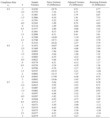
Table 3.4. Comparison adjusted variance estimates with naïve estimates and the variance estimated by bootstrap for the percentage difference from the sample variance of simulation: 2SRI approach with large sample size.
Compliance Rate C
ρ δ Variance Sample Naïve Estimate (% Difference) Adjusted Variance (% Difference) Bootstrap Estimate (% Difference)
0.3 -3 0.4105 -10.76 0.21 6.77
-2.5 0.3755 -7.16 2.71 5.56
-2 0.3401 -4.43 3.79 6.07
-1.5 0.3086 -4.10 1.91 7.53
-1 0.2701 -2.22 1.54 4.17
-0.5 0.2365 -1.09 0.79 4.65
0 0.2118 -1.09 -0.02 4.94
0.5 0.1977 -2.00 -0.08 5.42
1 0.1881 -0.13 4.49 7.35
1.5 0.2090 -8.31 0.41 5.81
2 0.2380 -14.60 -1.10 4.25
2.5 0.2740 -19.71 -1.64 5.70
3 0.3152 -24.26 -2.57 5.74
0.5 -3 0.1072 -10.07 -3.40 5.24
-2.5 0.1049 -9.98 -4.06 3.94
-2 0.0993 -7.86 -2.86 2.06
-1.5 0.0928 -5.64 -1.88 1.22
-1 0.0885 -6.55 -4.32 1.44
-0.5 0.0822 -5.68 -4.70 1.27
0 0.0778 -6.51 -6.12 1.17
0.5 0.0730 -5.24 -4.39 1.56
1 0.0706 -4.76 -2.17 1.20
1.5 0.0747 -10.35 -5.21 -1.04
2 0.0802 -15.15 -7.27 -1.76
2.5 0.0843 -17.09 -6.48 0.35
3 0.0882 -18.46 -5.65 0.79
0.7 -3 0.0416 -5.66 -3.43 0.70
-2.5 0.0415 -5.95 -3.91 0.73
-2 0.0407 -4.63 -2.85 0.82
-1.5 0.0402 -4.36 -2.95 0.93
-1 0.0397 -4.48 -3.52 1.67
-0.5 0.0387 -3.82 -3.33 2.38
0 0.0384 -4.92 -4.73 3.49
0.5 0.0372 -3.77 -3.58 3.27
1 0.0373 -5.59 -5.00 -1.13
1.5 0.0374 -6.85 -5.58 -0.92
2 0.0375 -7.46 -5.38 -1.20
2.5 0.0377 -8.23 -5.38 -1.18
3 0.0379 -8.73 -5.27 0.11
Note: Number of iteration of bootstrap p=700. Sample size N=1000, Simulation time M=2000.
Outcome rate for treatment group ω 11= ω 12= ω 13=0.6;