www.nat-hazards-earth-syst-sci.net/9/831/2009/ © Author(s) 2009. This work is distributed under the Creative Commons Attribution 3.0 License.
and Earth
System Sciences
Bayesian stochastic modeling of a spherical rock bouncing
on a coarse soil
F. Bourrier1, N. Eckert1, F. Nicot1, and F. Darve2
1Cemagref – UR ETNA, 2, rue de la Papeterie, BP 76, 38 402 Saint Martin d’H`eres Cedex, France 2L3S-R – INPG, UJF, CNRS, Domaine Universitaire, BP 53, 38 041 Grenoble Cedex 9, France
Received: 6 February 2009 – Revised: 4 May 2009 – Accepted: 20 May 2009 – Published: 10 June 2009
Abstract. Trajectory analysis models are increasingly used for rockfall hazard mapping. However, classical approaches only partially account for the variability of the trajectories. In this paper, a general formulation using a Taylor series ex-pansion is proposed for the quantification of the relative im-portance of the different processes that explain the variability of the reflected velocity vector after bouncing. A stochastic bouncing model is obtained using a statistical analysis of a large numerical data set. Estimation is performed using hier-archical Bayesian modeling schemes. The model introduces information on the coupling of the reflected and incident ve-locity vectors, which satisfactorily expresses the mechanisms associated with boulder bouncing.
The approach proposed is detailed in the case of the impact of a spherical boulder on a coarse soil, with special focus on the influence of soil particles’ geometrical configuration near the impact point and kinematic parameters of the rock before bouncing. The results show that a first-order expansion is sufficient for the case studied and emphasize the predomi-nant role of the local soil properties on the reflected velocity vector’s variability. The proposed model is compared with classical approaches and the interest for rockfall hazard as-sessment of reliable stochastic bouncing models in trajectory simulations is illustrated with a simple case study.
1 Introduction
Trajectory simulation models classically use Digital Eleva-tion Models that define the topography, and geographic in-formation systems that provide inin-formation on the rockfall sources and the spatial distribution of the parameters
neces-Correspondence to: F. Bourrier ([email protected])
sary to calculate the bouncing of the falling rocks at each point of the study site. The models classically used for bouncing calculations are based on restitution coefficients that express the dependence of the kinematic parameters of the rock after impact (reflected kinematic parameters) on the kinematic parameters of the rock before impact (inci-dent kinematic parameters). However, experimental studies have proved the complexity of simulating this dependence by means of reasonably simple mechanical models (Wu, 1985; Bozzolo and Pamini, 1986; Chau et al., 1998; Ushiro et al., 2000; Chau et al., 2002; Heidenreich, 2004). In addition, deterministic prediction of boulder bouncing remains highly speculative because the available information on the mechan-ical and geometrmechan-ical properties of the soil and the boulder is not sufficient. Indeed, the spatial distributions of the param-eters of the bouncing model integrated into the geographic information system result from a field survey which, for prac-tical reasons, cannot be exhaustive. Moreover, as for many physical processes in the field of natural hazards, it seems impossible to predict the bouncing deterministically.
Taking inspiration from other research fields such as hy-drology (Rao, 1996; Perreault et al., 2000a, 2000b) and avalanche science (Eckert et al., 2007, 2008) in which deal-ing with stochasticity is more common, this paper aims at defining a bouncing model explicitly distinguishing these different sources of variability.
In Sect. 2, a general framework that aims at determining the kinematics of the boulder after bouncing from the kine-matics before bouncing using a stochastic operator and its re-lated Taylor series expansion is presented first. This section also shows how the stochastic operator can be characterized using a Bayesian statistical analysis (Wickle, 2003; Clark, 2005) of numerical simulations. The study focuses on the impact of a boulder on a coarse soil, which is common in the context of rockfall trajectory analysis. In a first approxima-tion, only the influences of the incident kinematic parame-ters and the soil particle configuration near the impact point of a spherical boulder are studied. In Sect. 3, the stochastic bouncing model obtained using this approach is presented and discussed in detail. An extensive sensitivity analysis is performed to evaluate the bouncing model’s range of validity. Section 4 discusses the advantages and limitations of our ap-proach with regard to classical apap-proaches. The usefulness of using this stochastic bouncing model for the prediction of rockfall hazard is finally illustrated through a simple case study.
2 Materials and methods
2.1 Stochastic modeling of the impact
The bouncing model is developed in a two-dimensional frame, which is classical in the field of trajectory analysis (Guzzeti et al., 2002; Dorren et al., 2004). A generalized ve-locity vectorV composed of a normal-to-soil-surface veloc-ity componentvy, a tangential-to-soil-surface velocity com-ponentvx– both expressed at the gravity center of the falling rock – and a rotational velocityωproperly describes the kine-matic parameters of the boulder:
V = vxvy Rbω
t
(1) whereRbis the mean radius of the boulder.
For given mechanical and geometrical properties of the boulder and the soil, it is assumed that the incidentVinand reflectedVregeneralized velocity vectors of the boulder can be related by a stochastic operatorf˜:
Vre= ˜f (Vin) (2)
The formulation of the operatorf˜should express the com-plexity of the mechanisms leading to the dependence of the reflected velocity vector to the incident velocity vector. It should also be relevant for the variability of the bouncing process depending on the variability of the soil properties and the incident kinematic parameters.
Assuming that a Taylor series expansion of the operatorf˜ with respect to all components of the incident velocity vec-torVin exists, the operatorAcomposed of the coefficients of then-order Taylor series expansion off˜is defined. The operatorAassociates the reflected velocity vectorVrewith an incident velocity vector expressed asTin:
Vre=ATin+R (3)
with
A=
a1001 a0101 ... a1uvw... a10n0a100n a1002 a0102 ... a2uvw... a20n0a200n a1003 a0103 ... a3uvw... a30n0a300n
,
Tin=hvxinvyin...(vinx)u(vyin)v(Rbwin)w...(viny)n(Rbwin)ni t
,
u∈ [1, n], v∈ [1, n], w∈ [1, n],
andRa remainder term denoting the difference between the operatorf˜and its n-order Taylor series expansion. The num-ber of the incident vectorTincomponent is equal to 3 for a
first-order Taylor series expansion off˜, 7 for a second-order Taylor series expansion off˜, etc. One can note that, for a first-order Taylor series expansion of the operatorf˜, the in-cident vectorTinis equal to the incident velocity vectorVin. The high variability of the local configurations of the soil and the incident kinematic conditions induces the operator
Aand the remainder term R to take very different values. This suggests adopting a stochastic approach distinguishing the variability associated with both the operatorAand the remainder termR. Note that this paper only investigates in detail the case of the impact of a spherical boulder on a coarse soil. In a first approximation, the sources of variability con-sidered are limited to the incident kinematic parameters and the soil particles’ geometrical configurations. However, the proposed framework is very general and could be applied to modeling boulder bouncing for impacts on different soil types and for different boulder mechanical and geometrical properties. Indeed, as exemplified in this paper, it allows ex-tracting the respective contribution of the different sources of variability using Bayesian inference.
2.2 Data set definition from numerical simulations
The large data sets needed for statistical analyses can be ob-tained from numerical simulations of impacts. Additionally, in the simulations, the influences of the geometrical configu-ration of the soil near the impact point and the incident kine-matic parameters can be explored separately, since a precise and reproducible definition of these parameters is possible. 2.2.1 Numerical modeling of impacts using the Discrete
Element Method
the software Particle Flow Code 2-D (Itasca, 1999) based on the Discrete Element Method (Cundall and Strack, 1979) is used. In the Discrete Element Method (DEM), particles are subjected to gravitational forces and to contact forces. Con-tact forces are applied to neighboring particles in conCon-tact. For a given time step, once gravitational and contact forces have been computed, the translational and rotational veloc-ities of the particles are determined by solving the balance equation using an explicit solving scheme. The resulting particle displacements are used to update particle locations for the next time step. In this study, the contact forces act-ing between particles are calculated usact-ing the Hertz-Mindlin model (Mindlin and Deresiewicz, 1953). Contact forces are governed by three parameters set at classical values for rocks (Goodman, 1980): the shear modulus G is set at 40 GPa, the value of the Poisson ratioν is set at 0.25 and the local friction angleφis 30◦. In addition, the densityρof the boul-der and the soil particles is set at 2650 kg/m3. This contact model takes frictional processes between adjoining particles into account. Other dissipation sources also exist within real granular soils subjected to dynamical loadings, such as lo-cal yielding near the contact surface, crack propagation, and rock breakage. However, in the context of the simulations where a boulder is approximately of the same size as the soil particles, other dissipation sources can be assumed to be negligible compared to frictional dissipation in a first ap-proximation (Oger et al., 2005; Bourrier et al., 2008a).
The mean radius of the soil particles is Rm= 0.3 m. Given that natural scree are polydisperse granular assemblies (Kirkby and Statham, 1975), the ratio between the mass of the soil’s smaller particles and larger particles is set at 10. In the case of an impact on a coarse granular soil, boulder and soil particle sizes are nearly the same. The boulder radius Rbvaries fromRmto 5Rm. The influence of particle shape is also explored by defining two different soil samples com-posed of either spherical particles or elongated particles mod-eled by indivisible assemblies of spherical particles called clump particles, which can realistically model the shape of soil rocks (Bertrand et al., 2006; Deluzarche and Cambou, 2006; Bourrier et al., 2008a). The soil sample generation procedure leads to soil porosity values of 0.204 for spherical particles and 0.171 for clump particles. Additional details on the soil properties can be found in Bourrier et al. (2008a).
Although simulation results also depend on soil sample depth and porosity (Bourrier et al., 2008a), the influence of these parameters is not investigated in a preliminary approx-imation. Soil sample depth is set at 12Rm. Analyses of the influence of the model parameters on the impact simu-lations (Bourrier et al., 2008a) have shown that, for a soil depth corresponding to classical values in the field of rock-fall simulations, the bouncing of the boulder mainly depends on the ratio between the boulder radiusRb and the mean radius of a soil particleRm, the shape of the particles, the incident kinematic parameters and the geometrical configu-ration of the soil particles near the impact point. We will
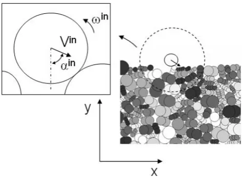
Fig. 1. Incident kinematic conditions.
focus on modeling the variability associated with the inci-dent kinematic parameters and the geometrical configuration of the soil particles near the impact point using a stochastic bouncing model (see Sect. 3). In addition, the influence of the ratio of the boulder radiusRbto the mean radius of a soil particleRmand the shape of the particles on the parameters of the stochastic bouncing model will also be investigated in Sect. 3 by means of sensitivity analyses.
Once the soil sample is generated, impact simulations are run for varying impact points and incident kinematic param-eters. The location of each impact point is defined very pre-cisely. In addition, incident kinematic conditions are fully determined by the magnitude of the incident velocityVin, the incident angleαinand the incident rotational velocityωin (Fig. 1). These parameters are directly related to the normal and tangential velocity components by:
vxin=Vinsin(αin) (4)
vyin= −Vincos(αin) (5)
Finally, reflected velocities are collected when the normal component of the boulder velocity reaches its maximum, which corresponds to the last contact between the soil and the boulder.
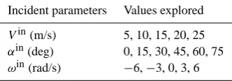
Table 1. Values of the incident kinematic parameters.
Incident parameters Values explored
Vin(m/s) 5, 10, 15, 20, 25
αin(deg) 0, 15, 30, 45, 60, 75
ωin(rad/s) −6,−3, 0, 3, 6
One limitation could stem from the differences in the sizes of the impacting and soil rocks during calibration and dur-ing application in this study. However, the influence of scale change effects was proved to be small by comparing the results of the numerical simulations of impacts at different scales (Bourrier, 2008). This has been confirmed by results from the literature in the field of aeolian sand transport (Oger et al., 2005).
2.2.2 Numerical simulation campaign
For given soil and boulder properties, several impact simula-tions were conducted for varying impact points and incident kinematic parameters. As stated above, the only sources of variability accounted for are the incident kinematic parame-ters and the soil particle geometrical configuration near the impact point. In addition, the dependency of the stochastic bouncing model parameter values on the boulder size and soil particle shape will be explored in Sect. 3.3. Other im-pact model parameters are set at fixed values: the mechanical properties of the particles (G,ν,φ,ρ), the porosity and grad-ing curve of the soil sample and the boulder size are fixed parameters.
Impact points are first precisely defined so that the same impact point can be used for several incident kinematic con-ditions: for a given impact point, a set of equally distributed incident kinematic parameters is explored. Kinematic pa-rameter values range within the limits defined from rockfall events (Azzoni et al., 1992). For each impact point, all com-binations of the chosen values for incident kinematic param-eters (Table 1) are explored. Preliminary numerical investi-gations have shown that a minimum ofP= 100 impact points has to be chosen to ensure that the mean values and standard deviations of the reflected velocity components (Bourrier et al., 2007) have reached their asymptotic value corresponding to the value obtained for very large numbers of impact points. 2.3 Stochastic analysis of simulation results based on
Bayesian inference
2.3.1 Hierarchical stochastic modeling
First, at each impact pointp∈[1, P], the Taylor series expan-sion (Eq. 3) of the operatorf˜defined in Eq. (2) is considered
a linear regression of the reflected velocity vectorVre with regard to the incident vectorTin:
Vrepk∼N3(ApTinpk,6) (6)
The reflected velocity Vre
pk is thus sampled from a local three-dimensional Gaussian vector fully defined by its lo-cal mean vectorApTinpk varying from one impact event to another and its covariance matrix6, which is constant for all incident kinematic conditionsk∈[1, K]and impact points (homoscedascity assumption). The vector ApTinpk is the mean predictor in the linear regression. Its variability quan-tifies the variability of the Taylor series expansion of f˜, while the covariance matrix6 accounts for the variability of the remainder term R. Our stochastic model is there-fore based on the assumption that the variability of the op-eratorAis only related with the variability of the soil parti-cles’ geometrical configuration, whereas the remainder term
R is associated with all other variability sources accounted for in the impact model, for instance random uncertainties that are not modeled explicitly. The realism of the me-chanical modeling representing the coupling between the re-flected and incident velocity vector depends on the order of the Taylor series expansion. For convenience, the matrix
Ap is rewritten as a vector having N components Alp =
h
a1001
pa010p
1...a1
uvwp...a0n0
1pa 00np
1a
1002p...a002npa1003p...
a00np
3
, with auvw1→3 denoting the coefficients of the matrix
A defined in Eq. (3) at the point p∈[1, P]. The number N=(n+1)(n+2)(n+3)/2–3 of the vector’s coefficients is equal to 9 for a first-order Taylor series expansion off˜(n=1), 27 for a second-order Taylor series expansion off˜(n=2), etc.
Second, it is assumed that the results observed at the dif-ferent impact points are, in some ways, similar because the macroscopic properties of the soil (porosity, the particles’ mechanical properties, grading curve, etc.) are the same. This makes us use hierarchical modeling to allow informa-tion to be partially shared between the different impact points and to extract the common patterns in all samples. For all im-pact pointsp, the coefficients of the operatorAp are there-fore assumed to be realizations of the same Gaussian vector such as:
A1p∼NN(Ma,6a) (7)
Ma and6a are the mean vector and the covariance matrix of theN-dimensional Gaussian vector.Mamodels the mean behavior all over the different local soil particles’ geometri-cal configurations, whereas the variability ofAl
p measured by6a expresses how close the different reflected velocities at the different impact points are.
contrary, even if it complicates model specification and in-ference, the hierarchical structure allows a comprehensive exploration of the grey zone situated between these two ex-treme cases. This makes each local estimation more robust and allows the overall quantitiesMaand6ato be captured.
The analytical formulation of the model developed can be summarized as follows. First, the analytical expression ofp(Vrepk
Ap,T
in
pk,6), the probability of the observed re-flected vectorVrepkknowing the values ofAp,6and the ob-served incident kinematic conditionsTinpkis:
p(Vrepk Ap,T
in
pk,6)=
1
(2π )3/2det(6)1/2e −12(Vre
pk−ApTinpk)t6
−1(Vre
pk−ApTinpk) (8)
Second, the analytical expression of the probability p(Alp|Ma,6a)of the nonobserved latent vectorAlp know-ing the values ofMa,6ais:
p(AlpMa,6a)=
1
(2π )N/2det(6a)1/2e −12(Al
p−Ma)t6a−1(Alp−Ma) (9)
The unknown parameters of the stochastic model are Ma,
6a, 6 and the data are Vre
pk andT
in
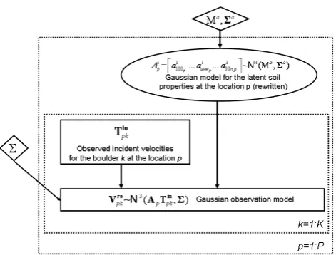
pk. The latent quanti-tiesAlp withp∈[1, P]have a hybrid status: with regard to the dataVrepkthey are parameters and therefore must be es-timated, whereas they behave as data with regard to param-etersMa and6a. Figure 2 gives a general overview of the model using a direct acyclic graph (DAG), which expresses conditional dependence. Circled nodes represent stochastic variables, while rectangles indicate observed values and di-amonds model parameters. The DAG clearly illustrates the three layers distinguished in our approach: impact that de-pends both on incident velocity and location, local soil con-figuration and the soil’s global parameters.
2.3.2 Bayesian inference
Due to its hierarchical nature, determining the parameters of our stochastic model using a classical statistical approach (Fischer, 1934; Neyman and Pearson, 1933) is tricky. On the other hand, estimates for the parametersMa,6aand6
and latent vectorsAlp,p∈[1, P]can be more easily obtained using Bayesian inference (Bayes, 1763). The result of apply-ing the Bayes theorem isp(Alp,Ma,6a, 6
V
re
pk,Tinpk), the joint posterior probability distribution of all model unknowns knowing the dataVrepkandTinpk:
p(Alp,Ma,6a,6
V
re pk,Tinpk)
=1
χp(M
a,6a,6)×p(Vre pk
Ap,T
in
pk,6)×p(Alp
Ma,6a)(10)
The determination of p(Alp,Ma,6a,6 V
re
pk,Tinpk) there-fore requires the probability of the reflected vector Vrepk
Fig. 2. DAG summarizing the hierarchical model.
knowing the data, latent variables Alp and the overall parameter 6 (p(Vrepk
Ap,T
in
pk,6)) and the probability p(Alp|Ma,6a) of the latent variables given the data and the overall parameters Ma,6a. Both of them are fully defined by the hierarchical model detailed in Sect. 2.3.1. Moreover, determining p(Alp,Ma,6a,6
V re
pk,T
in
pk) also requires specifyingp(Ma,6a,6).χ=R
p(Ma,6a,6)×
p(Vrepk Ap,T
in
pk,6) × p(Alp|Ma,6a)dMad6ad6 is a normalizing constant that does not depend on the problem’s unknowns, but makes all difficulty of Bayesian inference (see Sect. 2.3.3).
According to Bayesian interpretation,p(Ma,6a,6)is a prior, which is a probability distribution function that ex-presses the expertise about the parameters that is available before the data analysis. To respond to the classical objec-tions to use such prior information, in this paper we use poorly informative priors (Box and Tiao, 1973) that lead asymptotically to the same estimators as classical approaches (Berger, 1985). To facilitate inference using Gibbs sam-pling (see Sect. 2.3.3), the chosen poorly informative priors have been taken from conjugate families (see Gelman et al., 1995): a normal Gaussian vector with a null mean and very large variance forMa, and Wishart distributions with low de-grees of freedom for the inverse of the covariance matrixes (6,6a). Taking very poorly informative priors is possible since a data set as large as necessary is available given that numerical simulations were used to generate it. Poorly infor-mative priors have the advantage of letting the data speak for themselves so as to infer parameters with as much physical meaning as possible.
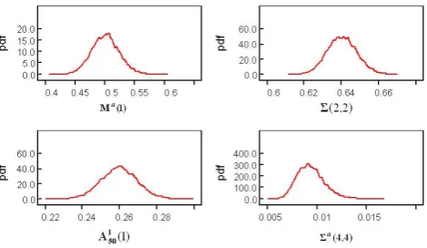
Fig. 3. Posterior distributions for a few unknown parameters.
mean of the posterior distribution and the 95% credible in-terval [q2.5, q97.5] are generally chosen for each unknown
pa-rameter, which represents the best prediction given the data and the related uncertainty. In this paper, this convention has been followed. In addition, the coefficient of variation cv defined as the ratio between the standard deviation and the mean value of the posterior distribution is also provided. It is a normalized measure of the dispersion of the posterior dis-tributions but has to be interpreted with care for disdis-tributions with small mean values.
2.3.3 MCMC methods
For hierarchical models, the computation of Bayes theorem is generally analytically unfeasible because of the problems calculating the normalizing constantχ. Today this limitation is routinely overcome, even for very complex models, with Monte Carlo techniques based on Markov chain properties (Brooks, 2003; Gilks et al., 2001). A general discussion of these Markov Chain Monte Carlo (MCMC) methods can be found in Robert and Casella (1998). Their aim is to obtain the posterior distribution of all model unknowns (parameters and latent variables) using an iterative procedure. Reason-able results can only be obtained if the algorithm is handled with care. In particular, one must ensure that the conver-gence is attained for all unknown parameters. In most cases, this requires launching many simulations for varying initial states and performing tests to check that the Markov chain has reached the stationary regime.
Depending on the model and the choice of priors, par-tial analytical computations can sometimes be performed for rather simple hierarchical models. This is the case for our model, given its fully Gaussian nature and the choice of con-jugate priors for all parameters. However, the full analytical expression of the joint posterior distribution remains out of reach, so that recourse to a simulation procedure is unavoid-able (see Gelman et al., 1995, chapter 15). It was therefore decided to perform a MCMC simulation for all unknowns, but to take advantage of the model’s structure by running the Gibbs sampler (Geman and Geman, 1984). This MCMC
al-Table 2. Posterior characteristics for a few unknown parameters.
Mean q2.5 q97.5 cv Ma(1) 0.5011 0.4560 0.5482 0.0468 Al50(1) 0.260 0.240 0.278 0.0378 6(2,2) 0.640 0.625 0.656 0.0124 6a(4,4) 0.00943 0.00707 0.0126 0.1476
gorithm is based on the different full conditional distributions of one unknown (parameter and latent variables) given the others, which can actually all be obtained with our model. The Gibbs sampler is particularly suitable because, when it can be run, it ensures a quick convergence with regard to the more general but less efficient Metropolis-Hastings al-gorithm (Metropolis et al., 1953). Note finally that, if the hierarchical structure is dropped by neglecting the random noise6, all computations can be performed analytically (see Sect. 3.2 for discussion).
For all the models tested (different orders of the Taylor se-ries expansion), 20 000 iterations were performed with dif-ferent chains starting at difdif-ferent points of the parameter space. The first 10 000 iterations were deleted to ensure that the ergotic state was attained. Convergence was checked for the second group of 10 000 iterations by comparing the dis-tributions obtained with the different chains. A few marginal posterior distributions are shown in Fig. 3 for the first-order model detailed in Sect. 3.2. For all parameters, the credibil-ity intervals obtained are small (Table 2). It therefore appears that the information conveyed by the data is sufficient and only the mean values and therefore be used with confidence. 2.3.4 Evaluation of model quality
The quality of the model is first evaluated by estimating the fraction of the variability of the reflected velocities that is captured by the random variableATincorresponding to the n-order Taylor series expansion off˜with regard to the total variability of the results. For thep-th impact point, thes-th component of the reflected velocity vectorVre and varying incident conditionsk, the ratiorps is calculated such that:
rps =
V (ApTinpk(s))
V (ApTinpk(s))+6(s, s)
(11)
calculated to estimate a mean percentage of variability ex-plained by the random variableATin for each reflected ve-locity component. In addition, an overall ratioris defined as the mean of allrps values.
3 Application to the definition and evaluation of a stochastic bouncing model
In this section, the statistical analysis of the data set obtained from numerical simulations is performed using the above-described procedure. This analysis allows defining a stochas-tic bouncing model and performing a detailed study of this model. All results obtained in this section are valid in the case of the impact of a spherical boulder on a coarse soil. In addition, the results obtained depend on the assumptions related to the numerical model of the impact, the procedure used for the numerical simulation campaign, and the statisti-cal analysis. The assumptions made during this analysis, the validity domain of the bouncing model obtained and the pos-sible generalization of this model for practical purposes will be discussed in Sect. 4.
3.1 A first-order model is sufficient
Several models corresponding to increasing dimensions of the incident vectorTinwere compared to determine the final formulation of the stochastic bouncing model. Particular at-tention was given to the precision and concision criteria since the bouncing model must satisfy a compromise between a precise simulation of the impact phenomenon and a small di-mension of the incident velocity vectorTin.
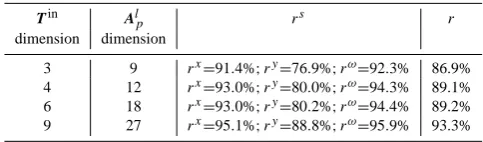
Table 3 summarizes the values of thers andr ratios for different models corresponding to increasing dimensions of the incident vectorTinin the case of the impact of a boulder with the radius set atRb=Rmon a soil composed of spher-ical particles. The size of the data set used was the same for all the models evaluated: 150 different incident kinematic conditions and 100 different impact points. The results first show that most of the variability of the reflected velocity is captured by the random variableATin for all models used
because therscoefficients are all greater than 75%.
Since all the models evaluated provide satisfying results in terms of precision, the most concise model was chosen: a dimension ofTinequal to 3, explaining most of the vari-ability of the results by the random variableATinfor a very small set of parameters. This model will hereafter be called the first-order stochastic bouncing model.
3.2 Detailed analysis of the first-order stochastic bouncing model
The model chosen corresponds to an incident vector Tin
composed of three components, which is equivalent to a
first-Table 3.rs andrvalues for increasing dimensions ofTin.
Tin Al
p rs r
dimension dimension
3 9 rx=91.4%;ry=76.9%;rω=92.3% 86.9% 4 12 rx=93.0%;ry=80.0%;rω=94.3% 89.1% 6 18 rx=93.0%;ry=80.2%;rω=94.4% 89.2% 9 27 rx=95.1%;ry=88.8%;rω=95.9% 93.3%
order Taylor series expansion of the stochastic operatorf˜:
vrex vrey Rbωre
∼N3(
a1a2a3
a4a5a6
a7a8a9
vxin vyin Rbωin
,
6xx 6xy 6xω 6xy 6yy 6yω 6xω6yω6ωω
)
(12) where the coefficients ai are sampled from a nine-dimensional Gaussian vector:
a1
... a9
∼N9(
ma1 ... ma9
,
611a ... 6a19 ... ... ... 619a ... 6a99
) (13)
This model separates the sources of variability for the re-flected velocity vector. The variability of parameters ai (i∈[1,9]) is quantified by the covariance matrix 6a. It is associated with the variations in the local soil properties. On the contrary, the variability quantified by the covariance ma-trix6 is related to the remainder term R and is therefore mainly associated with the incident velocities.
For the s-th component of the reflected velocity vector, the standard deviationes=
√
6ss of the regression residu-als provides a quantitative estimation of the proportion of the reflected velocity vector associated with the remainder term
R. The correlations between two componentssandtof the reflected velocity vector can be estimated by the linear cor-relation coefficientcst=√66st
ss6t t
∈[−1,1].
The estimates obtained show that, for all components of the reflected velocity vector, the standard deviation es is smaller than 1 m/s. Second, all the linear correlation coef-ficients range within the interval [−0.2,0.2], which means that the correlations between the components of the reflected velocity are small. The analysis of the covariance matrix6
Fig. 4. Marginal distribution of parametera2.
recent statistical developments. Indeed, ignoring the random noise6makes the model lose its hierarchical nature, so that the analytical expression of the posterior distribution is ac-cessible if the conjugate priors are kept forMaand6a.
Finally, the variability associated with the operatorAis estimated using the marginal normal probability distribution functions of parametersai (Fig. 4). The estimates for their mean valuesmai and standard deviationssia=p
6aiiare pro-vided in Table 4. Complementary to the marginal proba-bility distribution functions of each parameter ai, the cal-culation of the linear correlation coefficients cija = 6
a ij
q
6aij6ija (i∈[1,9];j∈[1,9])between the extra-diagonal terms of ma-trix6ashows strong correlations between parametersai be-cause thecija values are large.
3.3 Sensitivity analysis
3.3.1 Methodology for comparing the model’s parameters
To investigate the influence of several numerical simulation parameters, such as the number of impact points, the spa-tial distribution of soil particles, the value of the size ratio Rb/Rmand the shape of the soil particles, the parametersai obtained for different values of these simulation parameters must be compared.
The analysis is based on the marginal probability distri-bution functions of parametersai summed up by their mean valuemai and their standard deviation sai. Complementary to the qualitative comparison of the mean valuemai and the standard deviationsai obtained in the different cases, a com-parison criterionCi is calculated for each parameterai. The criterionCi evaluates the difference between the marginal distribution of parameterairefobtained using reference
con-Table 4. Mean valuesmai and standard deviationssai of parameters
ai.
mai sia
a1 0.5012 0.2412
a2 0.04167 0.2096
a3 −0.1598 0.0490
a4 0.2269 0.0971
a5 −0.07873 0.0640
a6 −0.03321 0.0428
a7 −0.4188 0.1130
a8 −0.04112 0.1809
a9 0.4439 0.0768
ditions and the marginal distribution of parameteracompi ob-tained using different numbers of impact points, different spatial distributions of the soil particles, different soil particle shapes or different boulder sizes. CriterionCi is calculated as follows:
Ci =
P (bi−≤aicomp≤bi+)−P (bi−≤airef≤bi+) P (bi−≤airef≤bi+)
(14) The lowerbi−and upperbi+bounds are calculated such that P (bi−≤airef≤bi+)=95% andP (arefi >bi+)=2.5%. Know-ing the values ofbi−andbi+makes it possible to determine the probability P (bi−≤aicomp≤bi+). The reference condi-tions correspond to the impact of a spherical boulder with its radius set atRb=Rmon a soil sample composed of spherical particles. The other properties of the soil sample are similar to those defined in Sect. 2.2.1. For the reference conditions, impacts are simulated on 100 different impact points. Cri-terion Ci can be interpreted as the difference between the most probable values of parameterai encountered with the reference conditions and the conditions evaluated for which only one simulation parameter (number of impact points, soil sample geometrical configuration, soil particle shape, boul-der radius) is changed compared to the reference conditions. 3.3.2 Robustness to simulation parameters
The first aim of this analysis is to quantify the number of sim-ulations necessary to obtain relevant values for parameters ai, which are therefore calculated using different numbers of impact pointsPfor the same soil sample. The analysis of the results obtained shows that the simulation onP= 20 differ-ent impact points is sufficidiffer-ent to obtain stable values for the probability distribution functions of parameterai. Indeed, all the values of criterionCi are less than 10% if the number of impact points is higher than 20 (Table 5).
Table 5. CriterionCifor different numbers of impact points.
C1 C2 C3 C4 C5 C6 C7 C8 C9
(%) (%) (%) (%) (%) (%) (%) (%) (%) 10 points −9 −2 −18 −4 −9 −17 2 −6 −14
20 points −1 −3 −9 0 −4 −6 0 0 −4
50 points 0 0 −2 −1 −1 −3 0 0 −2
(G,ν,φ,ρ). The only difference between the four samples is the spatial configuration of the particles. Soil sample no. 1 is the reference sample for the calculation of criterionCi.
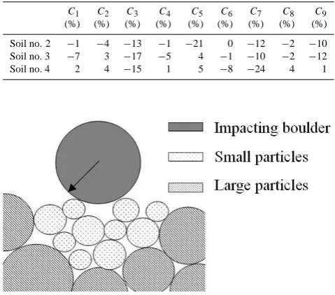
The results show that the sensitivity to the spatial configu-ration of the particles is relatively low for all the parameters (Table 6) because the maximum value obtained for criterion Ci is 24%. Greater differences are observed for parameters a3,a7anda9for whichCi reaches values greater than 10%
(respectively, 17%, 24% and 12%; Table 6). Moreover, the values of parametersaican locally be slightly different from all other values for a given soil sample. In this case, the value ofCi obtained for the considered sample is very dif-ferent from values obtained for all other samples. For ex-ample, the distribution of parametera5calculated using soil
sample no. 2 is very different from the other values obtained (C5= 21% for sample no. 2). A local analysis of the
geomet-rical configuration of the particles for sample no. 2 highlights the particles’ specific spatial distribution: several small par-ticles are located above larger parpar-ticles (Fig. 5). When the compression wave (Bourrier et al., 2008a) initiated at the be-ginning of the impact reaches the large particles, the energy is partially reflected toward the soil surface because of the larger inertia of the large particles. Supplementary kinetic energy is therefore transferred again to the boulder after en-ergy reflection, which leads to an increase in the reflected velocity and induces local changes in the values of parame-tera5.
3.3.3 Influence of the soil and boulder size
The influence of the characteristics of the soil and the boulder defines the model’s validity range. It is therefore essential for practitioners. Since an exhaustive parametrical study would be very long, the choice is made to limit the investigations to the influence of the parameters that are both accounted for in the impact model and commonly considered by practition-ers (Dorren et al., 2006). In most cases, for coarse soils, the available data are limited to the mean size and the shape of the soil particles. Additionally, in a preliminary approxima-tion, the influence of the geometrical and mechanical char-acteristics of the impacting boulder will not be studied. All simulations are therefore performed for the case of the im-pact of a spherical boulder.
To study the influence of soil particle shape, a set of pa-rameters ai is calculated using a soil sample composed of
Table 6. CriterionCifor different geometrical configurations of the soil particles.
C1 C2 C3 C4 C5 C6 C7 C8 C9
(%) (%) (%) (%) (%) (%) (%) (%) (%) Soil no. 2 −1 −4 −13 −1 −21 0 −12 −2 −10 Soil no. 3 −7 3 −17 −5 4 −1 −10 −2 −12
Soil no. 4 2 4 −15 1 5 −8 −24 4 1
Fig. 5. Local segregation of small particles above large particles.
In this configuration, a group of small particles is located above a group of large particles, whereas, in most cases, particles from different sizes are mixed.
clump particles with the same properties (see Sect. 2.2.1) as the reference soil sample. The results show that variations in the parameter values are significantly greater (Table 7) than the variations attributable to the geometrical configu-ration observed previously (Table 6). In particular, the cri-terionCi values (Table 7) exhibit significant differences for parametersa3,a4, a6, a8 anda9. These differences result
from differences in both the shape of the soil surface and the porosity of the soil. Indeed, using clump particles provides a more irregular soil surface composed of both quasi-planar and curved surfaces (Bourrier et al., 2007). It also induces smaller porosity values because the rearrangement of parti-cles is easier if the partiparti-cles have variable shapes (Bourrier et al., 2007).
The difference stemming from the use of spherical parti-cles cannot be considered insignificant. However, the results obtained using spherical particles provide a first-order ap-proximation of the reflected velocities for a very short com-putation time compared to simulations using clump parti-cles. Using spherical particles therefore provides an exten-sive parametrical analysis of the influence of the size ratio between the boulder and the soil particles.
Table 7. CriterionCi for a soil sample composed of clump parti-cles.
C1 C2 C3 C4 C5 C6 C7 C8 C9
(%) (%) (%) (%) (%) (%) (%) (%) (%)
−3 −2 −26 −15 −6 −27 −18 −12 −48
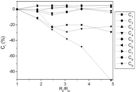
is analyzed by calculating the parameters of the stochastic bouncing model using a soil sample composed of spherical particles with a 2-D porosity of 0.204. TheRb/Rmratio of the boulder radius to the mean radius of the soil particles ranges within [1,5].
The values of the calculated criterionCi allow a compari-son of parametersaiobtained for differentRb/Rmratios with the parameters obtained for Rb/Rm=1, which correspond to parametersairef. The results show that the criteriaC5,C6
strongly depend on the value of theRb/Rmratio (Fig. 6) for 1≤Rb/Rm≤2.5 and that the criterionC9also strongly varies
depending onRb/Rmfor any value ofRb/Rm. From a prac-tical point of view, the variations observed clearly highlight that a single set of parametersai is not sufficient to model the impact on a given soil type for all boulder sizes. Differ-ent sets of parametersai have to be built, corresponding to differentRb/Rmratios.
4 Discussion
4.1 Comparison to classical approaches
The stochastic approach presented in this paper can be com-pared to classical approaches in the field of trajectory analy-sis. Classical models can be divided into several categories (Guzzetti et al., 2002) that consider the boulder either a sin-gle point or a rigid body. Moreover, some models differen-tiate two interaction types between the boulder and the soil: the falling rock can either roll or bounce onto the soil (Boz-zolo and Pamini, 1986; Evans and Hungr, 1993; Kobayashi et al., 1990; Azzoni et al., 1995), whereas most approaches consider boulder rolling a succession of small bounces. To model boulder bouncing, very complex bouncing models (Falcetta, 1985; Koo and Chern, 1998; Dimnet and Fremond, 2000) have been developed. They can describe the elastic, plastic, frictional or viscous dynamical behavior of the soil during impact. Although the differences between the previ-ously described approaches should not be omitted, the impact of the falling rock onto the soil is most often modeled using a tangential restitution coefficientet and a normal restitution coefficienten(Guzzetti et al., 2002):
et = v
re
x vin
x
(15)
Fig. 6. Influence of theRb/Rmratio on criterionCi.
en= vrey vin
y
(16)
The variability of the impact phenomenon is introduced as a last step by modeling the restitution coefficients and other parameters influencing the bouncing (Dudt and Heidenre-ich, 2001) as independent random variables that follow user-defined probability distribution functions (Dudt and Heiden-reich, 2001; Agliardi and Crosta, 2003; Frattini et al., 2008; Jaboyedoff et al., 2005) derived from back analysis of previ-ous events, experimental results or empirical expertise.
In our model, the mean predictor is the expected reflected velocity vectorE(Vre):
E(Vre)=
ma1vxin+ma2viny +ma3Rbωin ma4vxin+m5aviny +ma6Rbωin ma7vxin+ma8viny +ma9Rbωin
(17)
The usual restitution coefficientset andencan be compared to the tangential and normal components of the mean predic-torE(Vre)divided by the tangential or the normal compo-nents of the incident velocity vector, respectively:
et en
=
ma1 ma5
+
ma2v
in y
vin x
+ma3Rbωin
vin x
ma4vinx
vin y
+ma6Rbωin
vin y
(18)
The first term of Eq. (18) highlights that the mean pre-dictorE(Vre)is partially composed of a term equivalent to
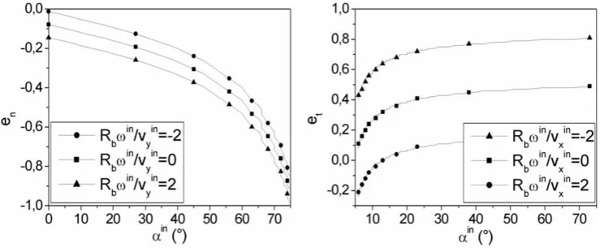
Fig. 7. Prediction of the model foret andenfor varying incidence anglesαinin and incident rotational velocitiesωin.
and other existing approaches is based on how this depen-dency is defined. In the proposed model, the dependepen-dency with the incidence angle is estimated from extensive statis-tical analysis, which allows exploring large impact configu-rations. On the contrary, in other existing approaches, this dependency was characterized from the physical analysis of experiments on smaller data sets that do not allow exploring the complete variability range of the reflected velocity.
Our stochastic bouncing model is therefore an extension of classical models that take into account the coupling between the incident kinematic parameters based on the analysis of the impact for very different incident kinematic conditions. The main difference between this model and the classical approaches is that the stochastic bouncing model is directly developed within an explicit stochastic framework. It there-fore allows modeling and quantifying correlations between the parameters that cannot be obtained if the variability of the impact phenomenon is introduced separately. A particularly notable characteristic of our approach compared to standard approaches is the hierarchical nature of the model that sep-arates the different sources of variability in the reflected ve-locity vector, for instance, the variability associated with the local characteristics of the impacted soil and with the boul-der’s incident kinematic parameters.
4.2 Remaining limitations and outcomes for further developments
Although comparing this model with classical approaches in the field of rockfall simulations is important, one has to keep in mind the assumptions and the restrictions associ-ated with the proposed stochastic bouncing model. These assumptions are related to the numerical impact model, the statistical analysis and the specificities of the case study for which the model was obtained.
The numerical impact model is a simplified simulation of the impact of a spherical boulder on coarse soils. Although the Discrete Element Method was proved to be relevant to model the impact, several assumptions were used during the modeling phase. As extensive numerical simulation cam-paigns were necessary, 2-D numerical simulations were per-formed although the impact is obviously a 3-D phenomenon. However, the half-scale experiments conducted to calibrate the model showed that the deviation of the rock from its inci-dent plane was fairly insignificant, which validates the use of 2-D simulations (Bourrier, 2008). The numerical model also implies a simplified simulation of all contacts between rocks (in particular, contact between the boulder and the soil parti-cles). Indeed, the model only accounts for energy diffusion inside the sample and for energy dissipation processes stem-ming from frictional processes. Other dissipation sources such as plastic dissipation at the contact points, the rocks’ partial or complete breakage fragmentation and elastic wave propagation are not accounted for in the model. Moreover, the fact that the model was calibrated from half-scale exper-iments and used for real-scale simulations could also be a limitation. However, investigations of the influence of scale changes made in this specific case study (Bourrier, 2008) and in other research fields (aeolian sand transport; see Oger et al., 2005) showed that scale change effects were very slight in this case. Finally, the impact model is only valid for a spher-ical boulder approximately the same size as the soil particle size, which corresponds to the case of a spherical projectile impacting a coarse soil. As mentioned above, despite these limitations, the results obtained in this study provide a basis for further simulation campaigns in which energy dissipation processes and impacting particle shape, in particular, would be modeled more precisely.
Fig. 8. Example study site.
distribution function. Since normal laws are defined over an infinite domain, the predictive use of the stochastic model can theoretically lead to the generation of negative values and large reflected velocities that would not be in accordance with energy conservation. However, given that the normal laws associated with parametersai exhibit little variability, the problem is not relevant in practice. On the other hand, the numerical simulation campaigns and statistical analyses performed only account for the variability associated with the local properties of the soil near the impact point and with the incident kinematic parameters. Additionally, the model parameters were determined for different values of the boul-der radius and for different soil particle shapes. The shape of the falling boulder, its orientation before impact, and the macroscopic properties of the soil (porosity,G,ν,φ,ρ, etc.) were not accounted for, although they are important sources of variability. The model obtained is therefore specific to a very particular configuration. However, the approach fol-lowed is a general framework for the precise characterization associated with each source of variability. It could be gener-alized over a large range of impact configurations to account for the above-mentioned effects. The main challenge would be to develop a relevant and numerical model of the impact for the different investigated configurations. It would then be necessary to calibrate it from real-scale experiments over a large range of incident conditions, which is obviously very difficult in practice.
Third, the specificities of the case study (impact of a spher-ical projectile on a coarse soil) induce several particularities in the bouncing model obtained. One can first note that a first-order Taylor series expansion of the stochastic opera-tor is sufficient to characterize boulder bouncing. Moreover, the variability associated with the remainder termRis very small. In the case of the impact on fine soils, the limitation to a first-order Taylor series expansion of the operator would certainly not be valid. Indeed, a first-order model does not account for the dependency of the reflected velocity on the magnitude of the incident velocity. It is truly insignificant for impact on coarse soils (Oger et al. 2005; Bourrier et al., 2007; Bourrier, 2008) but has been proven to be more sig-nificant in other cases such as the impact on fine soils (see Pfeiffer and Bowen, 1989; Heidenreich, 2004). In addition,
these particularities can be explained by the statistical anal-ysis being performed from numerical simulations that pro-vide a simplified vision of the “real” impact process. Finally, the results obtained would certainly be different if the influ-ence of the shape and orientation of the boulder were inte-grated. All these restrictions of the model provide interesting research topics for further studies.
4.3 Perspective for the predictive use of the model
The advantages of using the approach presented to properly model the variability associated with boulder bouncing in the field of rockfall hazard assessment are illustrated with a sim-ple 2-D examsim-ple.
In the example (Fig. 8), the study conducted aims at char-acterizing rockfall hazard on a homogeneous slope (100 m long, 35◦ slope) followed by a valley floor. The mean size of the soil particles is assumed to beRm= 0.2 m along the slope andRm= 0.1 m in the valley floor. The rockfall source, from which rocks detach starting with a 5-m-high freefall, is located at the top of the slope. The radius of the falling rocks is assumed to be 0.5 m.
The first advantages of using the approach proposed for rockfall simulations lie in the clear physical meaning of the parameters to be assessed in the field. In addition, the num-ber of parameters to be characterized in the field is reduced. Indeed, the validation of the stochastic bouncing model per-formed from real-scale experiments (Bourrier et al., 2009) showed that only theRb/Rmratio has to be characterized in the different zones of the study site. The other properties of the soil, such as substratum location (i.e., soil depth), poros-ity, and particle shape, can be set at fixed values for the entire site.
The integration of the stochastic bouncing model in a rock-fall trajectory simulation model is based on the definition of a database composed of several sets of parametersai for vary-ing values of theRb/Rm ratio. The porosity of the soil, its depth and the particles’ shape at the study site must also be evaluated. For each bouncing calculation, the reflected ve-locity vector is calculated from the incident veve-locity vector by using the stochastic bouncing model predictively. The values of parametersai to be used for each bouncing calcu-lation are determined depending on the value of theRb/Rm ratio. A field survey must therefore be conducted to assess the spatial distribution ofRmover the study site. Addition-ally, the boulder radiusRbalso has to be evaluated for each rockfall simulation.
Fig. 9. DistributionP (x|D)depending on the horizontal distancex
from the rockfall source.
P(x|D) for the rock, once detached, to propagate through the locationx(see Jaboyedoff et al., 2005, for example), such as:
H (x)=P (D)P (x|D) (19)
The calculation of the detachment probability P(D) is not within the scope of this study. On the other hand, the use of the stochastic bouncing model can be highly advanta-geous for a reliable estimation of the cumulative distribution P (X≥x|D)=P (x|D)for the rock to exceed the abscissax. The probabilityP (X≥x|D)=P (x|D)is calculated by inte-grating the discretized density p(x, y, Ec) of the falling rock passing through the point(x, y) with a kinetic energyEc, which is a direct outcome of trajectory simulations:
P (x|D)=P (X≥x|D)= ∞ Z
0
∞ Z
0
∞ Z
x
p(x, y, Ec|D)dxdydEc (20)
In the example considered here, a total of 10 000 trajectory simulations are performed following the above-described procedure. The decrease in the probability P(x|D) depend-ing on the distancex from the release point (Fig. 9) shows that most of the falling rocks reach the valley floor because P(x|D) is greater than 85% forx≤82 m. However, as soon as the valley floor is reached, the probability P(x) of a rockfall event occurring sharply decreases with distancex. In partic-ular, it is smaller than 10% forx>120 m.
Additionally, using a reliable local discretized density p(x, y, Ec|D) means the rockfall hazard can be studied more pre-cisely. It is, for example, possible to determine a 2-D map that defines the probability for the occurrence of rockfall events at all points of the study site. In a 2-D context, this information is associated with the following probability: P (x, y|D)=P (X≥x, y−δy/2< Y ≤y+δy/2|D)
Fig. 10. DistributionP (x, y|D) for the occurrence of a rockfall event at all points of the study site.
= ∞ Z
0
y+δy/2 Z
y−δy/2 ∞ Z
x
p(x, y, Ec|D)dxdydEc (21)
whereδy is the vertical size of the cells resulting from the discretization of the study site.
Figure 10 provides an illustration of this type of 2-D map for the example. To compute this map, the horizontalδx and the verticalδy cell sizes associated with the discretization of the study site are set at 1 m. Figure 10 clearly shows that most of the falling rocks propagate near the slope’s surface. In addition, forx<80 m, the most probable trajectories are located at increasing distances from the slope’s surface when altitude decreases. This indicates that, on a steep constant slope, materials at risk such as electric cables situated far from the release zone can be hit even if they are situated far above the soil surface. However, as soon as the valley floor is reached, the altitude range containing most of the trajectories substantially decreases whenx increases because gravity no longer compensates energy dissipation at each impact.
Note that a simple hazard assessment procedure has been used in this example. However, more advanced guidelines could have been implemented, since p(x, y, Ec|D) is the ba-sis of all methods used for rockfall hazard characterization. Since the flight phase of the rock is deterministic, the rele-vance of the probability p(x, y, Ec|D) is determined by the accuracy of the bouncing model. This fully justifies the use of the stochastic bouncing models, which suitably account for the variability associated with different sources.
distribution of the rocks’ energy when impacting the struc-ture, which will be investigated in further work.
5 Conclusions
In this paper, a general framework was proposed for the char-acterization of the variability of falling boulders’ velocities after rebound. The use of large data sets from numerical im-pact simulations and of Bayesian modeling schemes has led to the definition of a stochastic bouncing model in the context of the impact of a spherical projectile on a coarse soil. This stochastic bouncing model uses a hierarchical structure that can quantify the relative importance of different contribu-tions to the reflected velocity vector’s variability. This model also introduces couplings between the reflected and incident velocity vector that are sufficient to model the mechanism associated with boulder bouncing.
The detailed analysis of the model has proved its relevance for modeling the variability of the reflected velocity vector for all spatial configurations of the soil particles. In addi-tion, the parametrical study conducted demonstrated that the model is valid for different values of the boulder size to soil mean particle size ratio and for different soil particle shapes. The comparison with classical bouncing models in the field of trajectory analysis highlighted that the model can be con-sidered an extension to classical models that accurately in-tegrates the couplings between the reflected and the incident kinematic parameters. Moreover, it has been shown that for the impact of spherical boulders on coarse soils, first-order Taylor series expansion on the incident velocity is sufficient to express of the variability of the reflected velocity. An-other important result is that, in this case, the variability of the local soil configurations strongly dominates random un-certainties. On the other hand, the model is able to take into account the couplings between the model’s parameters that stem from the mechanical complexity, and our results have indicated that they should not be neglected.
From a practical point of view, the bouncing model devel-oped can easily be integrated into rockfall simulation codes that model trajectories of spherical boulders. The main ad-vantages of this procedure compared to classical approaches, which generally require field assessment of the parameters, is that the required input parameters have a clear physical meaning.
In the future, our procedure could be used to characterize the bouncing of a boulder on all different types of soil sur-face, such as fine soils or rocky surfaces, with the possible inclusion of field observations and real-world data using the chosen Bayesian approach (Straub and Schubert, 2008). Our approach could also be used to characterize the variability associated with other important variability sources of boul-der bouncing, such as boulboul-der shape. The challenge would then be to provide large data sets composed of reproducible and precisely defined results. For this purpose, the direct
use of experimental results is not suitable. On the contrary, like the methodology proposed here, data sets could be gen-erated from numerical simulations. Finally, as illustrated in the case study, the stochastic bouncing model proposed can be used for prediction purposes, making a consistent prob-abilistic starting point available for carrying out prediction-oriented simulations of boulders impacting a coarse soil. In particular, it can be used to build multivariate probability dis-tribution functions characterizing hazard levels on an endan-gered slope and to compute risk levels taking at-risk struc-tures into account.
Edited by: A. Volkwein
Reviewed by: D. Straub and another anonymous referee
References
Agliardi, F. and Crosta, G.: High resolution three-dimensional nu-merical modelling of rockfalls, Int. J. Rock Mech. Min., 40, 455– 471, 2003.
Azzoni, A., Rossi, P. P., Drigo, E., Giani, G. P., and Zaninetti, A.: In situ observation of rockfall analysis parameters, in: Proceedings of the sixth International Symposium of Landslides, Rotterdam, The Netherlands, 1, 307–314, 1992.
Azzoni, A., Barbera, G., and Zaninetti, A.: Analysis and predic-tion of rockfalls using a mathematical model, Int. J. Rock Mech. Min., 32, 709–724, 1995.
Bayes, T.: Essay towards solving a problem in the doctrine of chances, Philos. T. R. Soc. Lond., 53 and 54, 370–418 and 296– 325, 1763.
Berger, J. O.: Statistical Decision Theory and Bayesian Analysis. 2nd edn., Springer-Verlag, 1985.
Bertrand, D., Nicot, F., Gotteland, P., and Lambert, S.: Modelling a geo-composite cell using discrete analysis, Comput. Geotech., 32, 564–577, 2006.
Bourrier, F., Nicot, F., and Darve, F.: Rockfall modelling: Numer-ical simulation of the impact of a particle on a coarse granular medium, in: Proceedings of the 10th International Congress on NUmerical MOdel in Geomechanics, edited by: Pietruszczak, S. and Pande, G., Taylor & Francis, 699–705, 2007.
Bourrier, F.: Mod´elisation de l’impact d’un bloc rocheux sur un terrain naturel, application `a la trajectographie des chutes de blocs, Ph.D. thesis, Institut Polytechnique de Grenoble, Greno-ble, France, 2008.
Bourrier, F., Nicot, F., and Darve, F.: Physical processes within a 2D granular layer during an impact, Granul. Matter, 10(6), 415–437, 2008a.
Bourrier, F., Eckert, N., Bellot, H., Heymann, A., Nicot, F., and Darve, F.: Numerical modelling of physical processes involved during the impact of a rock on a coarse soil, in: Proceedings of the conference Advances in Geomaterials and Structures, edited by: Darve, F., Doghri, I., El Fatmi, R., et al., Collection S.T, 501–506, 2008b.
Box, G. E. P. and Tiao, G. C.: Bayesian inference in statistical anal-ysis, Addison-Wesley, 1973.
Bozzolo, D. and Pamini, R.: Simulation of rock falls down a valley side, Acta Mech., 63, 113–130, 1986.
Brooks, S. P.: Bayesian Computation: A Statistical Revolution, Transactions of the Royal statistical society, Series A, 2681– 2697, 2003.
Chau, K. T., Wong, R. H. C., and Lee, C. F.: Rockfall Problems in Hong Kong and some new Experimental Results for Coefficients of Restitution, Int. J. Rock Mech. Min., 35(4–5), 662–663, 1998. Chau, K. T., Wong, R. H. C., and Wu, J. J.: Coefficient of restitution and rotational motions of rockfall impacts, Int. J. Rock Mech. Min., 39, 69–77, 2002.
Clark., J. S.: Why environmental scientists are becoming Bayesians, Ecol. Lett., 8, 2–14, 2005.
Cundall, P. A. and Strack, O. D. L.: A discrete numerical model for granular assemblies, Geotechnique, 29, 47–65, 1979.
Deluzarche, R. and Cambou, B.: Discrete numerical modelling of rockfill dams, Int. J. Numer. Anal. Met., 30, 1075–1096, 2006. Dimnet, E. and Fremond, M.: Instantaneous collisions of solids, in:
Proceedings of the European Congress on Computational Meth-ods in Applied Sciences and Engineering, Barcelona, Spain, 11– 17, 2000.
Dorren, L. K. A., Maier, B., Putters, U. S., and Seijmonsbergen, A. C.: Combining field and modelling techniques to assess rockfall dynamics on a protection forest hillslope in the European Alps, Geomorphology, 57(3), 151–167, 2004.
Dorren, L. K. A., Berger, F., and Putters, U. S.: Real-size ex-periments and 3-D simulation of rockfall on forested and non-forested slopes, Nat. Hazards Earth Syst. Sci., 6, 145–153, 2006, http://www.nat-hazards-earth-syst-sci.net/6/145/2006/.
Dudt, J. P. and Heidenreich, B.: Treatment of the uncertainty in a three-dimensional numerical simulation model for rock falls, in: Proceedings of the International Conference on Landslides – Causes, Impacts and Countermeasures, Davos, Switzerland, 507–514, 2001.
Eckert, N., Parent, E., and Richard, D.: Revisiting statistical-topographical methods for avalanche predetermination: Bayesian modelling for runout distance predictive distribu-tion, Cold Reg. Sci. Technol., 49, 88–107, 2007.
Eckert, N., Parent, E., Naaim, M., and Richard, D.: Bayesian stochastic modelling for avalanche predetermination: from a general system framework to return period computations, Stoch. Env. Res. Risk A., 185–206, 2008.
Evans, S. and Hungr, O.: The assessment of rockfall hazard at the base of talus slopes, Can. Geotech. J., 30, 620–636, 1993. Falcetta, J. L.: Un nouveau mod`ele de calcul de trajectoires de blocs
rocheux, Revue Franc¸aise de G´eotechnique, 30, 11–17, 1985. Fischer, R. A.: Probability, likelihood and quantity of information
in the logic of uncertain inference, P. Roy. Soc. A, 146, 1–8, 1934.
Frattini, P., Crosta, G. B., Carrara, A., and Agliardi, F.: Assessment of rockfall susceptibility by integrating statistical and physically-based approaches, Geomorphology, 94(3–4), 419–437, 2008. Geman, S. and Geman, D.: Stochastic Relaxation, Gibbs
Distribu-tion and the Bayesian RestoraDistribu-tion of Images, IEEE T. Pattern Anal., Pami-6, 6, 721–741, 1984.
Gelman, A., Carlin, J. B., Stern, H. S., and Rubin D. B.: Bayesian Data Analysis, Chapman & Hall, New-York, USA, 1995.
Gilks, W. R., Richardson, S., and Spiegelhalter, D. J.: Markov Chain Monte Carlo in Practice, Chapman & Hall, New-York, USA, 2001.
Goodman, R. E.: Introduction to rocks mechanics, PWS Publishing Company, Boston, USA, 1980.
Guzzetti, F., Crosta, G., Detti, R., and Agliardi, F: STONE: a com-puter program for the three dimensional simulation of rock-falls, Comput. Geosci., 28, 1079–1093, 2002.
Heidenreich, B.: Small and half scale experimental studies of rock-fall impacts on sandy slopes, Ph.D thesis Ecole Polytechnique F´ed´erale de Lausanne, Lausanne, 2004.
Itasca Consulting Group.: PFC2D User’s manual, Itasca, Min-neapolis, USA, 1999.
Jaboyedoff, M., Dudt, J. P., and Labiouse, V.: An attempt to refine rockfall hazard zoning based on the kinetic energy, frequency and fragmentation degree, Nat. Hazards Earth Syst. Sci., 5, 621–632, 2005, http://www.nat-hazards-earth-syst-sci.net/5/621/2005/. Kirkby, M. and Statham, I.: Surface stone movement and scree
for-mation, J. Geol., 83, 349–362, 1975.
Kobayashi, Y., Harp, E. L., and Kagawa, T.: Simulation of Rock-falls triggered by earthquakes, Rock Mech. Rock Eng., 23, 1–20, 1990.
Koo, C. Y. and Chern, J. C.: Modification of the DDA method for rigid blocks problems, Int. J. Rock Mech. Min., 35(6), 683–693, 1998.
Labiouse, V. and Descoeudres, F.: Possibilities and Difficulties in predicting Rockfall Trajectories, in: Proceedings of the Joint Japan-Swiss Scientific Seminar on Impact Load by Rock Falls and Design of Protection Structures, Kanazawa, 29–36, 1999. Metropolis, N., Rosenbluth, A. W., Rosenbluth, M. N., Teller, A. H.,
and Teller, E.: Equation of State Calculations by Fast Computing Machine, J. Chem. Phys., 21, 1087–1091, 1953.
Mindlin, R. D. and Deresiewicz, H.: Elastic spheres in contact un-der varying oblique forces, J. Appl. Mech., 20, 327–344, 1953. Neyman, J. and Pearson, E. S.: On the testing of statistical
hypoth-esis in relation to probability a priori, Proc. Camb. Philos., 29, 492–510, 1933.
Oger, L., Ammi, M., Valance, A., and Beladjine, D.: Discrete El-ement Method to study the collision of one rapid sphere on 2D and 3D packings, Eur. Phys. J. E, 17, 467–476, 2005.
Paronuzzi, P.: Probabilistic approach for design optimization of rockfall protective barriers, Quaterly Journal of Engineering Ge-ology, 22, 175–183, 1989.
Perreault, L., Bernier, J., Bob´ee, B., and Parent, E.: Bayesian change-point analysis in hydrometeorological time series. Part 1. The normal model revisited, J. Hydrol., 235(3–4), 221–241, 2000a.
Perreault, L., Bernier, J., Bob´ee, B., and Parent, E.: Bayesian change-point analysis in hydrometeorological time series. Part 2. Comparison of change-point models and forecasting, J. Hydrol., 235(3–4), 242–263, 2000b.
Pfeiffer, T. and Bowen, T.: Computer Simulation of Rockfalls, Bul-letin of the Association of Engineering Geologists, 26(1), 135– 146, 1989.
Rao, A. and Tirtotjondro, W.: Investigation of changes in charac-teristics of hydrological time series by Bayesian methods, Stoch. Env. Res. Risk A., 10(4), 295–317, 1996.
Straub, D. and Schubert, M.: Modelling and managing uncertainty in rock-fall hazards, Georisk, 2(1), 1–15, 2008.
Ushiro, T., Shinohara, S., Tanida, K., and Yagi, N.: A study on the motion of rockfalls on Slopes, in: Proceedings of the 5th Sym-posium on Impact Problems in Civil Engineering, Japan, 91–96, 2000.
Wikle, C.: Hierarchical Bayesian models for predicting the spread of ecological processes, Ecology, 84, 1382–1394, 2003. Wu, S. S.: Rockfall evaluation by computer simulation, Transport.