Copyright by author(s); CC-BY 1679 The Clute Institute
IPO Waves: How Market Performances
Influence The Market Timing Of IPO?
Firas Batnini, Ph.D., ESSCA School of Management, FranceMoez Hammami, Statistician Economist Engineer at Lunalogic, France
ABSTRACT
The goal of this paper is to study the impact of stock markets on Initial Public Offerings (IPOs). Several studies have shown that the need for financing is not the main trigger for an IPO— favorable market conditions may play a more important part. This work prove the existence of a significate relationship between past stock market returns and the number of IPOs. Before setting the date for an IPO, managers analyze long term financial market yields, a bullish stock market over a six month/ one year period encourages IPOs activities. In the other hand, even a negative performance but over a two-year period may have the same effect. They expect a stock market inversion. These results were obtained by autocorrelation analysis and count regression.
Keywords: IPO; Stock Market Performance; Autocorrelation; Count Regression; Main Component Analysis
INTRODUCTION
n Initial Public Offering or IPO aims above all at raising funds which will thereby enable a firm to recapitalize or finance its expansion. It also builds on a firm’s visibility and notoriety and offers shareholders greater liquidity. However, the constraints linked to such an operation (cost, loss of power for managers, disclosure of sensitive information, and so on) can sometimes go beyond the operation’s advantages. In this case why then do corporations carry out IPOs? Benniga et al. (2005), having studied the optimal conditions for an IPO, concluded that investment financing is not reason enough to launch an IPO.
The scientific literature tends more and more to consider the thesis of market timing which encourages many firms to precipitate their IPO decision (Baker and Wurgler, 2002). According to Lowry (2003), economic recovery and investor optimism can encourage a corporation to launch an IPO. Thus, the IPO decision is influenced both by exogenous economic conditions and by a firm’s own financing needs. Lerner et al. (2003) showed that in very unfavorable market conditions where introduction price are weak, only those corporations who had urgent short-term financing needs or future high-yielding projects would accept to launch an IPO. The search for the optimal moment to carry out an IPO conduct to remark empirically periods of weak IPO concentrations and other periods of busy concentration. This empirical assessment of IPO market dynamics is known by the name “IPO Waves:” a wave of strong activities (known as a “hot” market) is generally followed by a wave of less intense (“cold” market) activities.
Van Bommel and Vermaelen’s (2003) work determined that the most undervalued companies and those that accepted to carry out an IPO in a cold market phase are also those that invested the most post-IPO. Undervaluation is an introductory cost for corporations with a real financing need and which cannot put off their IPOs until the optimal conditions have been reached. Moreover, Alti (2005) confirmed that companies having launched an IPO during a hot market phase retained more financing in their cash flows than those having carried one out in a cold market period. Those firms did not show a real need for financing but took advantage of auspicious timing to raise funds. Finding genuine motivation for an IPO is correlative to determining influencing factors in the emergence of IPO waves.
of daily IPOs and stock market yields. Finally, the fourth section presents the count regression model used and the main results.
REVIEW OF THE LITERATURE
According to the literature, the most influential factors in the birth of IPO waves are:
- Technological change and the emergence of followers/copiers; - Data asymmetry;
- Capital market yields.
Technological Change and innovation
The arrival of new technology demands very fast development and requires considerable investment. According to Stoughton et al. (2001), if a leading corporation—meaning one which holds the patent to or initiated the original technology—decides to launch an IPO, it provides sufficient information on its future cash flow, which enables investors to better assess the sector. Other (follower/copier) firms profit from this opportunity to launch an IPO. This theory was confirmed by Lowry (2003) who proved that technological shock created significant capital needs and drove several companies to launch an IPO with an aim to raise funds. However, this theory was contradicted by Helwege and Liang (2004) who found that technological innovation is not unique among hot market contexts and thus does not make up the main determining factor in IPO waves as IPO cycles are more frequent than innovation cycles. In the end, technological change does not fully explain IPO waves but rather the arrival of other firms seeking out capital. This example can be seen in internet firms in the 1990s, followed by biotechnology companies and more recently by social networks. Competition on the stock market means that investors are becoming scarcer and late arrives will not be able to access the market under the right conditions (Hsu et al. 2010).
Data Asymmetry
Other theories explain IPO waves, by a high level of market data asymmetry (Choe et al., 1993; Rajan and Servaes, 1997 and 2003; Lowry, 2003). The number of IPOs increases when stocks are overvalued. Initial past IPO yields play the role of indicator for corporate heads seeking to find out if the time is right for them to carry out an IPO (Benveniste et al., 2003). Banks play a vital role in the spread of information, and during hot market phrases, they demand even more data from the companies involved to facilitate the operation (He, 2007). Other corporate heads, upon detecting overvalued IPO prices, profit from the opportunity to speed up their own IPOs and raise a larger amount of funds than had been originally planned. However, the firstcomers to the market have an advantage in reputation which enables them to earn market shares in comparison to the followers (Chemmanur and He, 2011).
If the average IPO price exceeds analysts’ forecasts, then IPO volumes will mark a strong increase. A high IPO price sends a positive signal to the market, which will encourage those companies waiting for the right moment to launch an IPO to decide to risk lowering the number of shares issued and thus the capital they raise, and increase the probability of abandoning the operation (Boch and Dunbar, 2014). According to Yung et al. (2008), IPOs carried out during hot market phases are associated with a higher yield variance and buyout rate than normal. For a corporate decision maker or an investor, it is safer to analyze the standard deviation of the initial yield to find out whether the price is over- or undervalued (Lowry et al., 2011). Nonetheless, this theory has its limits, notably because the decision to launch an IPO is not short term, but prepared over a much longer period; therefore other explanations of these concentration phenomena exist.
Capital Market Yields
Copyright by author(s); CC-BY 1681 The Clute Institute Pastor and Veronesi (2005) noticed that IPO waves are preceded by an increase in market yields and followed by decreases. IPO concentrations appear as soon as forecasts begin predicting an increase in expected yields. Thus, the decision to launch an IPO is comparable to an American call. The value of the option depends on the market. It increases if the market level increases. When the market value increased substantially over the past two years, investors forecast a market reversal in a near future and a strong decrease (of the market and thus of their option). This then is the right moment for a firm to call its option and launch an IPO. The work of Loughran et al. (1994) confirmed this idea by showing that market levels (the option’s delta) and its volatility (the vega) had a positive effect on the number of IPOs.
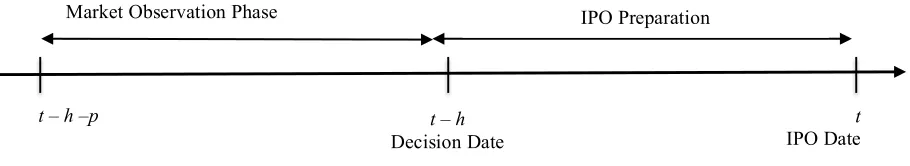
These studies confirm the intuitive notion of the impact of capital market variation on IPO waves. However, the lead-lag effect between the number of IPOs and market performance has been the object of little research. An IPO is not an instantaneous operation; it requires a certain amount of legal, financial and organizational preparation, which is why an IPO is generally decided on several months prior to the actual launch. Let us suppose that an IPO is carried out at a given t moment. The decision for the IPO was made h weeks prior to t (i.e. the t-h moment). If this decision was motivated by the observation of the stock market, then the company’s directors followed its performance during p weeks (between the t-h-p moment and the t-h moment). Figure 1 illustrates this decision making process.
Figure 1. The IPO Process
This article has two main goals:
- Checking that corporate heads observe stock market trends before deciding on an IPO.
- Measuring and assessing the range of preparation (the h parameter) and the market observation (the p parameter) phases.
DATA AND WORKING METHODOLOGY
Data
We chose to focus our attention on the following two series:
- The series of weekly IPO numbers (nbIPO) carried out between January 1, 2000 and December 31, 2011 on the American market.
- The series of weekly yields of S&P500 market index.
This choice was motivated by the ambition to determine the lead-lag effect between the number of IPOs and market yields only (the S&P index often being considered as a proxy for American stock markets). The remaining factors which may have weighted this relationship were implicitly considered as residue.
Weekly IPO Numbers Series
The initial data series comes from the NYSE Euronext database1. It represents all IPO operations carried
out on the American market over the 2000-2011 period. This series is made up of 2307 observations. We aggregated them week by week to obtain the series of weekly IPOs which we then carried over to the nbIPO figure. This new series included 628 observations.
1 The NYSE Euronext IPO database is available at: https://europeanequities.nyx.com/fr/listings/ipo−showcase
Market Observation Phase IPO Preparation
t – h –p t – h
Decision Date
Graphically (Figure 2), we were able to single out periods of intense activity as in 2000 and 2006, and other periods of weaker activity as for example in 2001 and 2008. These IPO waves correspond to hot market and cold market periods.
Figure 2. Weekly IPO Series
On average, more than three IPOs (3.15 exactly) were recorded weekly with a standard deviation of nearly 4 (3.95) IPOs. The fact that the average is higher than the mean (equal to 2), that the asymmetrical coefficient is positive (Skewness=1.91) and that the kurtosis is high (excess kurtosis2 =4.64) confirms even more the existence of
IPO waves since we have noticed several weeks of very high activity and others where activity is very low.
The S&P500 Yield Series
The S&P500 (SPX) is a market index based on the quotes of the 500 largest American firms. It is often considered as the most representative stock market indicator in the United States.
Figure 3 shows the index’s cumulative yields for the period covering 2000-2011. The annualized yield over this period is equal to -0.99%, annualized volatility at 20.69% and the Sharpe ratio at -0.04. In essence, this period was bearish at a total of -15%. However, we also noticed several other trends:
- Strong decrease between 2000 and 2001 corresponding to the burst in the internet bubble; - Recovery from 2002 until end 2007;
- Decrease due to the 2008 recession; - Recovery from end 2008.
Thus, over the course of the survey, stock markets went through two major recessions due to the dot-com bubble burst (2001) and the sub-prime crisis (2008), as well as two successive recoveries. This aspect is noteworthy to our work in that we were able to detect the impact of strong market variations on the number of IPOs.
Copyright by author(s); CC-BY 1683 The Clute Institute Figure 3. S&P500 Cumulative Yield, 2000-2011
Methodology
The purpose of our work is to explain the series of IPO numbers (nbIPO) via the series of market yields and their lags3 (past series of yields). Integration of these delayed series allowed us to investigate the lead-lag between
these two variables. We created P series of cumulative yields over periods of one week to P weeks: from the S&P500 weekly yields, we calculated the cumulative yield series over p weeks with p ∈ [1, P]. These series were then noted in the rest of the article Rt(p) and defined according to the following formula:
Rt(p) = )*+( r#$%,#$%'(
Where rt – i, t – i +1 = ln ,,-./01
-./ represented the weekly return of the index over the period [t − i, t − i + 1].
Since yields are continuous, the series of cumulative yields R(p) corresponded to the index returns over the last p weeks.
Rt (p) = )*+( r#$%,#$%'( = ln ,-./01
,-./ )
*+( = ln
,-./01
,-./ ,
*+( = ln ,,-.4- = rt – p, t
To investigate the relation between the number of IPO and the S&P lagged returns, we have implemented two different methods. The first method consisted in calculating and testing the statistical significativity of cross-autocorrelation coefficients between the nbIPOt series and the cumulative Rt–h (p) series for different parameters h
[0, H] and p ∈ [1, P]. It thus enabled us to determine the h and p parameters which influenced IPO decision making process, h being the length (in weeks) before the actual launch (in t) and p being the length (in weeks) of the yields observed at the t-h moment. For example, suppose that we find a significantly positive correlation for the parameters (p = 50 and h ∈ [10, 20]). There is thus a significantly positive correlations between the number of IPOs at moment t (nbIPOt) and the yields over 50 weeks calculated at (t-10, …, t-20). We may then conclude that the managers, at
the moment they made the IPO decision, took into account the S&P500 yields over 50 weeks and their decision was made between 10 and 20 weeks prior to the IPO launch.
The second method consisted of building a regression model explaining the IPO number (nbIPO) via a series of market yields and their lags. However, it is not possible to use a linear regression model for the following technical reasons:
- The number of IPOs being a count variable, linear regression models are not applicable. - Cumulative yield series are, by nature of their construction, highly correlated since
Rt(p) = Rt(p - 1) + r#$5,#$5'(, ∀p ∈ [1, P ] et ∀t ∈ [1, T ].
- The number of explicative variables is too high: we have at our disposal P series of cumulated yields and H delayed series for each of them. If we consider, for example, P = H = 104, there will be 10,920 explicative variables.
Thus we set up the following methodology:
- Use a count regression model, more adapted to the type of explained variable to explain (Colin et al., 2013);
- Use a dimension reduction technique as principal component analyses (PCA) reduce the number of explicative variables and guarantee the orthogonality of the explicative variables.
CROSS-AUTOCORRELATION
Definition
Cross-autocorrelation is the linear correlation coefficient between two temporal series Xt and Yt and their
respective lags. If we consider k lags we obtain the cross-autocorrelation matrix M sized of (2k + 1, 2k + 1) with the following coefficients:
Mij = corr (Xt − i, Yt − j) with i ∈ [−k, k] and j ∈ [−k, k]
In our study we were interested in analyzing the relationships between the number of IPOs (nbIPOt) and the
series of cumulated yield (Rt-h(p)) for the different delays h ∈ [0, H] and the different lengths p ∈ [1, P].
Thereafter, we calculated for each p parameter the CP = (cp,0, ..., cp,h, ..., cp,H) vector with
cp,h = corr (nbIPOt, Rt − h(p))
All the vectors formed the cross-autocorrelation C matrix whose size was (P, H + 1).
Cross-Autocorrelation Matrix
Copyright by author(s); CC-BY 1685 The Clute Institute Figure 4. Auto-Correlation Matrix. h is the length (in weeks) before the actual
IPO launch (in t) and p the length (in weeks) of the yields observed in t-h.
We can make out three areas. These areas are distinct enough from each other and may be interpreted as follows:
1. The pink area (positive correlation). This area corresponds to lags under 52 weeks (h < 52) and cumulated yields over a period higher than 12 weeks (p > 12). This shows that managers analyzed the S&P 500 returns for the IPO throughout the preceding year (h < 52) over periods of between 3 and 24 months (p > 12).
2. The light blue area (absence of correlation). This area corresponds to the cumulated yields over a short period (p < 12) and this for all lags (∀ h ∈ [0,104]). It suggests that managers in the decision making process were not interested in short-term market yields. They were interested in longer trends.
3. The dark blue area (negative correlation). This area corresponds to delays above 70 weeks (h > 70) and the cumulated yields over a rather long period (p > 40). This shows that managers were anticipating a stock market shift whereas past S&P500 returns (over 70 weeks, or more than one year and four months) were negative. These yields were calculated over a rather long period (medium to long-term yields).
The detected areas enable us to conclude that managers:
- They sought seeking to detect a possible market inversion to prepare an IPO. For example if the market had been bearish for more than a year, the directors would have begun scheduling the IPO date one and a half years later, because they would have believed that over the course of that time the market would have recovered.
- They continued to analyze market performance over an average period of two years (parameter p) and between six months and one year prior to the date of the IPO (parameter h). This survey allowed them to confirm the IPO decision or to postpone it.
- We suppose that managers follow short-term market performance during the year prior to the IPO launch to quantify the number of shares to issue during the IPO and to help them set the IPO price, but did not influence the actual IPO decision.
Correlation Intensity
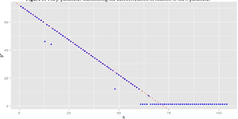
p* (h) = argmax corr [(nbIPOt, Rt−h(p))] with p ∈ [1,P]
Figure 5 shows the results obtained. The abscissa shows the h lag parameter and the ordinate the p* parameter.
Figure 5. The p parameter maximizing the autocorrelation in relation to the h parameter
The relation between the p* and h parameters is a decreasing linear relation on the h ∈ [0, 60] interval. The equation of this line is approximated by:
p* = K – h, with K = 72
This relation can be interpreted in the following way:
- If the operator decides to carry out the IPO, h weeks before the launch, s/he will first analyze the market performances over a period of (72 – h) weeks. Generally, the IPO decision comes 3 to 6 months before the actual launch, according to our results. Managers thus analyze market performance between 10 and 13 months (between 46 and 59 weeks) before the date on which the decision is made.
- The linear relation shows that managers continue to follow the state of the markets. For example, if they begin following the stock market six months prior to the IPO, they will be interested in market trends over the past 10 months. They will continue watching the market up to the IPO and the determination of the IPO price.
The analysis of correlation intensity enabled us to deduce that managers follow the market continuously before the IPO.
COUNT REGRESSION
Model and Methodology
The IPO number series (nbIPO) represents a series of counting data. The linear regression model is not suited to this type of data4. A more adapted model is the Poisson regression. Let us consider a counting data Y as the
4 The variable to be explained (nbIPO) is supported in ℕ whereas the linear regression was adapted to continuous support variables (ℝ for
Copyright by author(s); CC-BY 1687 The Clute Institute explained variable (Y∈ℕ) and X = (x1,…,xK) as the explaining variables (X ∈ℝK). Y follow a poisson law with λ
parameter. The poisson model consists in carrying a linear regression on the 𝔼 (Ln(y)) as follow:
Ln (E(Y)) = ln(λ) = β0 + β1x1 + ... + βk xk + u Where (β0,…,βK) are the regression coefficients
The model coefficients are estimated by maximum likelihood under certain hypotheses. They are not respected in our case for two reasons: the over-dispersion (Variance > Average) and the colinearity of the independent variables. In the rest of this section we will present these problems and the proposed solutions.
The Dispersion Problem:
The Poisson regression model is based on the following implicit hypotheses:
- Events happen at a constant rate. - Events are independent.
In practice, it is rare that the event independence hypothesis is respected. In our case, for example, we expected that the occurrence of an IPO would increase the probability of other IPOs taking place (contagion effect), thus triggering hot market and cold market phases. If this hypothesis was broken, an over dispersion phenomenon took place: the variance of the observed events went beyond its expectation (contrary to the Poisson model characteristics). This problem was corrected by the quasi-Poisson model (For more information on poisson models and quasi-poisson correction, see Ver Hoef and Boveng, 2007) : the dispersion effect was corrected by introducing a new θ parameter in the variance variable:
Y : V(Y) = 𝜃λ with 𝜃 > 1
The Multi-Colinearity Problem in the explaining Variables:
By construction, our explaining variables—cumulated yields Rt(p)—are multi-colinear since Rt(p) =
Rt(p−1)+rt-p,t-p+1. To solve the colinearity problem, we carried out a Prinicpal Component analysis (PCA). This
dimension reduction method provides the following two advantages:
- Orthogonality: the axes obtained via PCA are, by construction, orthogonal (independent).
- Reduced dimensions: the selection of the first PCA axes enabled us to reduce the number of explaining variables.
Principal Components Analysis (PCA)
The PCA was carried out on the temporal Rt(p) series, ∀p ∈ [1,P] for the period of January
2001-December 2011. (628 observations5). P was fixed at 104.
Selection of the Number of PCA Axes
Analysis of the contribution of each PCA axis to the total inertia (variance) enabled us to select the number of axes to retain. The first axis explained 69.06% of the total inertia. The second axis explained 14.45% of this factor, and the third 5.58%. The other axes (a total of 101) explained 2.83% at best and overall 10.89%.
According to the traditional selection methods (the elbow method), it is recommended to select the first two PCA axes. Together, they explain 83.51% of the total variance. The third axis only explains a small proportion of the total variance: 5.6% or twice less than the second axis and 12 times less than the first. We analyzed these axes to
understand their meanings and interpret them, since the PCA axes—linear combination of initial variables—had no real meaning as the latter (cumulated yields).
PCA Axis Interpretations
The first axis represents 69% of the total variance. The projections of all the variables on this axis are negative. This axis thus represents a leveling effect. We compared these coefficients to the average cumulated yields R(p) = (A AC+(𝑅C 𝑝 , the maximum cumulated yields (max(R(p)) = max(R1(p), ..., RT (p))), and the absolute value of
the maximum cumulated yields (max(|R(p)|) = max(|R1(p)|, ..., |RT (p)|)). We carried out linear regressions of the cumulated yields and time periods:
R(p) = α0,p + α1,pt + up
The comparison between the time coefficient (αl,p representing the time trend) and the coefficient of the
first axis (c1,p) show that they are opposed ∀p ∈ [1, P] (at the nearest multiplicative constant as shown in Figure 7).
Figure 7. PCA first axis coefficients compared to those in the cumulated yield regression in relation to time
We thus consider the first axis as that of the “opposite trend,” which may be interpreted as follows:
- A positive value on this axis shows the existence of a negative trend; - A negative value on this axis shows the existence of a positive trend.
Copyright by author(s); CC-BY 1689 The Clute Institute Figure 8. Coefficients of the Second MCA Axis
The first two PCA axis, represent the trend and the maturity. The space them may be interpreted as follows:
- Upper left region: short term positive trend - Upper right region: short term negative trend - Lower left region: long term positive trend - Lower right region: long term negative trend
In the rest of this work, we explained the IPO number (nbIPO) via the P =< Axe1, Axe2 > plan and it different lags. This enabled us to comprehend and quantify the lead time between market observation and the IPO decision date. The regression model we retained took the following shape:
NbIPO = f (< Axis1, Axis2 >0,…...,< Axis1, Axis2 >h)
Modelling of the =< Axis1, Axis2 > plan can be done in several different ways:
- < Axis1, Axis2 >= Axis1 + Axis2: As in the two independent Axis with absolutely no interaction (even in time).
- < Axis1, Axis2 >= Axis1 + Axis2 + Axis1 * Axis2: By adding consideration for the interaction of the two Axis. However, this modelling represented a redundancy in information (the two Axis were modelled as well as their interactions).
- < Axis2, Axis2 >= Axis1 + Axis1 * Axis2: taking the interaction into account, while deleting the information redundancy.
- < Axis1, Axis2 >= Axis2 + Axis1 * Axis2: same modeling as before but keeping axis2 instead of axis1.
The third and fourth models are equivalent. We retained the third model as we think that the effect of the first axis is more important than that of the second considering the inertia that it explains.
Count Regression
The variable to be explained is the weekly IPO number (nbIPO). The explanatory variables are: the P =< Axis1, Axis2 > plan made up of the first two axes of the PCA and represented by Axis1 + Axis1 * Axis2, and its H lags. Our overall model is thus written:
nbIPO = P0 + P1 + ... + PH + u
Where Pi represents the plan delayed by i periods: Pi = Axis 1i + (Axis1 * Axis 2)i; H is set at 104 weeks and u
represents the regression residue.
The average number of weekly IPOs is around 3 whereas the variance is 13, a figure which empirically confirms the presence of the problem of over-dispersion6. This problem will be handled by using the quasi-Poisson
correction as previously explained.
The number of independent variables being rather high (210 independent variables7), we wished to reduce this figure by selecting the best lagged plans. This simplified comprehension of the model, but also avoided the colinearity problem between the P =< Axis1, Axis2 > plan and its delays. To select the best models, we used the selection algorithm proposed by Famoye and Rothe (2003) and adapted especially for count regressions. The algorithm was modified to select only the <Axis1, Axis2> plan each time instead of only one variable.
The measurement used to select the best model is deviance. It measures the quality of model adjustment by comparing its log-likelihood to that of the full model (with all explanatory variables). The model with the smallest deviance is the model retained. Afterwards, for each q size of the retained sub-group, we obtain an “optimal” model, i.e. one with the least deviance. Table 1 presents the optimal models for each q size.
Table 1. Optimal models for each explanatory plan sub-group
q Deviance Selection
1 1 733.98 p 2
2 2 680.64 p 2, p 100
3 3 660.97 p 2, p 100, p 98
4 4 650.64 p 2, p 100, p 98, p 1
5 5 645.26 p 2, p 100, p 98, p 1, p 14
We carried out the different regressions proposed and selected the most sparing model, whose coefficients are significant at the 5% threshold. The model retained is:
nbIPO = p2 + p100
Or nbIPO = Axis12 + Axis12 * Axis22 + Axis1100 + Axis1100 * Axis2100
Table 2. Regressions Results
Coefficients Estimate Std. Error T value Pr(>𝒕)
(Intercept) 0.7745183 0.0862469 8.980 < 2e − 16 ***
Axis1.2 -0.1374036 0.0143546 -9.572 < 2e − 16 ***
Axis1.100 -0.0290960 0.0059316 -4.905 1.29e-06 ***
Axis1.2*Axis2.2 0.0097789 0.0028229 3.464 0.000581 ***
Axis1.100*Axis2.100 -0.0024159 0.0009595 -2.518 0.012137 *
Signif. codes: 0 ‘***’ ; 0.001 ‘**’ ; 0.01 ‘*’ ; 0.05 ‘.’
Copyright by author(s); CC-BY 1691 The Clute Institute We noticed that:
- For plan 2 (two weeks before the IPO): the coefficient of Axis1 is negative, therefore we followed positive trends. The coefficient of the product of Axis1*Axis2 is positive so we followed long term trends. The positive long term trends at two weeks until the IPO pushed managers to carry out the launch.
- For the 100 plan (100 weeks or nearly two years before the IPO), Axis1 coefficient is negative (positive trend). The coefficient of the product of Axis1*Axis2 is also negative, meaning that short term trends will be followed: two years before the IPO a positive short term trend (market inversion?) will push directors to launch the IPO. This result can be interpreted as an indication that directors, following a long downward period, expect stock market inversion and thus a recovery of growth, which should increase the number of IPOs and create a hot market.
The analysis of the model’s standardized residues shows that the model does not present any too-frequent extremes. We noticed that the extreme residues are positive; this showed that our model underestimated the weeks where the number of IPOs was too high (see Figure 9). This can be explained by firms which had a real need for financing and did not carry out Market Timing.
Figure 9. Number of weekly IPOs carried out (in black) and the number of forecast IPOs (in green) according to count nbIPO = Plan2 + Plan100
CONCLUSION
Several papers dealt with managers’ motivation on carrying out an IPO despite market constraints and shareholder demands. What kept our attention was that several authors proved that financing needs did not make up the sole reason for this decision (Benninga et al., 2005). Market timing plays an important part in the choice of IPO scheduling (Baker and Wugler, 2002). Market recovery and resurgence in optimism may encourage some directors to rush their decisions if they are searching for the right time frame for their IPO, a theory confirmed by Lowry (2003). This theory though is limited: during recessions, only those firms who are facing urgent financing needs carry out IPOs (Lerner et al., 2003).
Count regression enabled us to confirm the existence of a link between the decision to launch an IPO and past market yield. Two years prior to the IPO, a positive short term trend favored IPO markets. It represented the beginning of a market turnaround. In conclusion, we can state that the two methods led to the same conclusion—the existence of a strong relation between IPO waves and market performance. We noticed that directors observed market changes prior to making their decision as to the date of the IPO launch. The observation period was over p weeks, and they began their observations with a period of h weeks before the launch, this date corresponding to the moment the decision to launch was made. Generally, the trigger for this decision is a forecasted increase in the market for the period covering the IPO. This materialized through a market decrease over the weeks of observation, at the end of which the markets generally turned themselves around, this moment being the best for directors to launch the IPO. After this decision was made, the directors never stopped observing the markets; for a period corresponding to P, they were still able to postpone the IPO if they noticed that the market did indeed not recover.
AUTHOR INFORMATION
Firas Batnini, Ph.D., Department of Finance, ESSCA School of Management, France. E-mail: Firas.batnini@essca.fr
Moez Hammami, Department of MSc Statistics and MSc Management, Statistician Economist Engineer at Lunalogic, France. E-mail: Moez.hammami@lunalogic.com
REFERENCES
Alti, A. (2005). Ipo market timing. The Review of Financial Studies, 18, 1105-1138.
Baker, M. P., & Wurgler, J. (2002). Market timing and capital structure. Journal of Finance, 57, 1-32.
Benninga, S., Helmantel, M., & Sarig, O. (2005). The timing of initial public offerings. Journal of Financial Economics, 75, 115–132.
Benveniste, L.M., Ljungqvist, A.P., Wilhelm, Jr. W.J., & Yu, X. (2003). Evidence of information spillovers in the production of investment banking services. Journal of Finance, 58, 577–608.
Boeh, K., & Dunbar, C. (2014). IPO waves and the issuance process. Journal of Corporate Finance, 25, 455–473.
Chemmanur, T.J., & HE, J. (2011). IPO waves, product market competition, and the going public decision: Theory and evidence.
Journal of Financial Economics, 101, 382–412.
Choe, H., Masulis, R., & Nanda V. (1993). Common stock offerings across the business cycle: theory and evidence. Journal Empirical Finance, 1, 3–31.
Colin, A. C., & Pravin, K. T. (2013). Regression Analysis of Count Data. Cambridge University Press.
Famoye, F., & Rothe, D.E. (2003). Variable Selection for Poisson Regression Model. Journal of Modern Applied Statistical Methods, 2, 380-388.
He, P. (2007). A Theory of IPO Waves. The Review of Financial Studies, 20, 983-1020.
Helwege, J., & Liang N., (2004). Initial public offerings in hot and cold markets. Journal of Financial and Quantitative Analysis, 39, 541-569.
Hsu, H.C., Reed, A., & Rocholl, J. (2010). The new game in town: competitive effects of IPOs. Journal Finance, 65, 495–528. Lerner, J., Shane, H., & Tsai, A. (2003). Do equity financing cycles matter?: evidence from biotechnology alliances. Journal of
Financial Economics, 67, 411–446.
Loughran, T., Ritter, J., & Rydqvist K. (1994). Initial public offerings: international insights. Pacific-Basin Finance Journal, 2, 165–199.
Lowry, M. (2003). Why does IPO volume fluctuate so much? Journal of Financial Economics, 67, 3-40.
Lowry, M., Officer, M., & Schwert, G.W. (2011). The variability of IPO initial returns. Journal of Finance, 65, 425–465. Pastor, L., & Veronesi, P. (2005). Rational ipo waves. Journal of Finance, 60, 1713-1757.
Ritter, J. R., & Welch, I. (2002). A Review of IPO Activity, Pricing, and Allocations. Journal of Finance, 57, 1795-1828. Rajan, R., & Servaes, H. (1997). Analyst following of initial public offerings. Journal of Finance, 52, 507-530.
Rajan, R., & Servaes, H. (2003). The effect of market conditions on initial public offerings. In: McCahery, J., Renneboog, L. (Eds.), Venture Capital Contracting and the Valuation of High-tech Firms. Oxford University Press, 18, 437-463. Stoughton, N. M., Wong, K. P., & Zechner, J. (2001). IPOs and product quality. Journal of Business, 74, 375-408.
Van Bommel, J., & Vermaelen, T. (2003). Post-Ipo capital expenditures and market feedback. Journal of Banking and Finance, 58, 1499-1520.
Ver Hoef, J. M., & Boveng, P. L. (2007). Quasi-Poisson vs. negative binomial regression: how should we model overdispersed count data?. Ecology, 88, 2766-2772.