Embodied Visual Perception Models For Human Behavior Understanding

(1)

University of Pennsylvania

ScholarlyCommons

Publicly Accessible Penn Dissertations

2019

Embodied Visual Perception Models For Human

Behavior Understanding

Gediminas Bertasius

University of Pennsylvania, [email protected]

Follow this and additional works at:

https://repository.upenn.edu/edissertations

Part of the

Artificial Intelligence and Robotics Commons

Recommended Citation

Bertasius, Gediminas, "Embodied Visual Perception Models For Human Behavior Understanding" (2019).Publicly Accessible Penn Dissertations. 3344.

(2)

Embodied Visual Perception Models For Human Behavior Understanding

Abstract

Many modern applications require extracting the core attributes of human behavior such as a person's attention, intent, or skill level from the visual data. There are two main challenges related to this problem. First, we need models that can represent visual data in terms of object-level cues. Second, we need models that can infer the core behavioral attributes from the visual data. We refer to these two challenges as ``learning to see'', and ``seeing to learn'' respectively. In this PhD thesis, we have made progress towards addressing both challenges.

We tackle the problem of ``learning to see'' by developing methods that extract object-level information directly from raw visual data. This includes, two top-down contour detectors, DeepEdge and Hf L, which can be used to aid high-level vision tasks such as object detection. Furthermore, we also present two semantic object segmentation methods, Boundary Neural Fields (BNFs), and Convolutional Random Walk Networks (RWNs), which integrate low-level affinity cues into an object segmentation process. We then shift our focus to video-level understanding, and present a Spatiotemporal Sampling Network (STSN), which can be used for video object detection, and discriminative motion feature learning.

Afterwards, we transition into the second subproblem of ``seeing to learn'', for which we leverage first-person GoPro cameras that record what people see during a particular activity. We aim to infer the core behavior attributes such as a person's attention, intention, and his skill level from such first-person data. To do so, we first propose a concept of action-objects--the objects that capture person's conscious visual (watching a TV) or tactile (taking a cup) interactions. We then introduce two models, EgoNet and Visual-Spatial Network (VSN), which detect action-objects in supervised and unsupervised settings respectively. Afterwards, we focus on a behavior understanding task in a complex basketball activity. We present a method for evaluating players' skill level from their first-person basketball videos, and also a model that predicts a player's future motion trajectory from a single first-person image.

Degree Type

Dissertation

Degree Name

Doctor of Philosophy (PhD)

Graduate Group

Computer and Information Science

First Advisor

Jianbo Shi

Keywords

(3)

Subject Categories

(4)

EMBODIED VISUAL PERCEPTION MODELS FOR HUMAN BEHAVIOR UNDERSTANDING

Gediminas Bertasius

A DISSERTATION

in

Computer and Information Science

Presented to the Faculties of the University of Pennsylvania

in

Partial Fulfillment of the Requirements for the

Degree of Doctor of Philosophy

2019

Supervisor of Dissertation

Jianbo Shi, Professor of Computer and Information Science

Graduate Group Chair

Rajeev Alur, Zisman Family Professor of Computer and Information Science

Dissertation Committee

Kostas Daniilidis, Ruth Yalom Stone Professor of Computer and Information Science

Camillo J. Taylor, Professor of Computer and Information Science

(5)

(6)

ACKNOWLEDGEMENT

For many students, PhD can be a frustrating and a lonely experience. Not only does it

require extraordinary amounts of persistence, but also a substantial amount of luck. Over

my five years, I observed that students who make it through their PhD typically have a very

strong support system around them. I am no exception in this regard, and I attribute my

overwhelmingly positive PhD experience to all the people who helped me reach this point.

First, I would like to thank my advisor Jianbo Shi for giving me full intellectual freedom to

pursue any research interests that I was drawn to during the last five years. Jianbo’s faith in

me allowed me to work on many new and interesting problems, most of which later resulted

in solid publications. Jianbo also taught me how to approach and formulate new research

problems, which I think is one of the most invaluable skills that I learned throughout my

PhD. Finally, I am thankful to Jianbo for always being supportive, especially after the

negative paper reviews. His positivity during those times pushed me to work harder and

eventually get those papers accepted to subsequent conferences. Overall, my PhD journey

has been very fulfilling, and I am grateful to Jianbo for this experience.

I would also like to give a big thanks to Lorenzo Torresani, who is one of the main reasons

why I pursued a PhD in the first place. Lorenzo sparked my interest in computer vision

re-search during my undergraduate years at Dartmouth, and I’ve stayed in the field ever since.

I was lucky to continue collaborating with Lorenzo during my PhD years, and I learned a

great deal from Lorenzo about various research methodologies, experimental design, and

technical writing. His guidance over all these years significantly contributed to my success,

and I will always be grateful for his mentorship.

I am also grateful to Hyun Soo Park, and Stella Yu. I learned a lot from both of them.

Hyun Soo taught me how to effectively sell my research ideas to other people both in writing

and in presentation. I think these were truly invaluable lessons, that allowed me to publish

(7)

my research from a different perspective, and how to present it more effectively to broader

audiences who have different backgrounds than my own.

I would also like to express my gratitude for everybody involved in the IGERT program.

Being part of IGERT weekly meetings, allowed me to broaden my research horizons and

think about my research in the context of other fields such as psychology, robotics, and

human vision. During IGERT meetings, I had a great pleasure to observe Kostas Daniilidis’,

and David Brainard’s discussions about research, and learn from both of them. Kostas

and David consistently gave me useful feedback, and helped me to think critically about

the broader impact of my work. A special thanks to Kostas for the basketball related

discussions, which always brightened my mood.

I am also thankful to my other dissertation committee member CJ Taylor for his insightful

comments and suggestions in regards to my research. I appreciated CJ’s attention to detail,

his thought provoking questions, and his kind personality. It was truly a pleasure having

him on my dissertation and my WPE II committees.

Another big thanks goes to the Facebook’s AI Applied Research team, who made my

summer internship experience fruitful and enjoyable. In particular, I want to thank Lorenzo,

Du Tran, and Christoph Feichtenhofer who were my mentors during the internship. Each

of them has taught me something unique about video understanding research, and helped

me to become a better researcher. I’d also like to give a special thanks to a fellow intern

Antoine Miech who kept both of our spirits high throughout the internship.

Finally, I wanted to thank my parents Rima, and Gintaras, and my wife Alex for always

supporting me. From the early age when my main priority was basketball, my parents

always stressed the importance of education and encouraged me to excel in both of these

areas, which led me to where I am now. Additionally, my wife Alex was the most ardent

believer of my success, which inspired me to accomplish any goals that I set out for myself.

(8)

ABSTRACT

EMBODIED VISUAL PERCEPTION MODELS FOR

HUMAN BEHAVIOR UNDERSTANDING

Gediminas Bertasius

Jianbo Shi

Many modern applications require extracting the core attributes of human behavior such

as a person’s attention, intent, or skill level from the visual data. There are two main

challenges related to this problem. First, we need models that can represent visual data

in terms of object-level cues. Second, we need models that can infer the core behavioral

attributes from the visual data. We refer to these two challenges as “learning to see”, and

“seeing to learn” respectively. In this PhD thesis, we have made progress towards addressing

both challenges.

We tackle the problem of “learning to see” by developing methods that extract object-level

information directly from raw visual data. This includes, two top-down contour detectors,

DeepEdge [1] and HfL [2], which can be used to aid high-level vision tasks such as

ob-ject detection. Furthermore, we also present two semantic obob-ject segmentation methods,

Boundary Neural Fields (BNFs) [3], and Convolutional Random Walk Networks (RWNs) [4],

which integrate low-level affinity cues into an object segmentation process. We then shift

our focus to video-level understanding, and present a Spatiotemporal Sampling Network

(STSN), which can be used for video object detection [5], and discriminative motion

fea-ture learning [6].

Afterwards, we transition into the second subproblem of “seeing to learn”, for which we

leverage first-person GoPro cameras that record what people see during a particular activity.

We aim to infer the core behavior attributes such as a person’s attention, intention, and

(9)

action-objects–the objects that capture person’s conscious visual (watching a TV) or tactile (taking

a cup) interactions. We then introduce two models, EgoNet [7] and Visual-Spatial Network

(VSN) [8], which detect action-objects in supervised and unsupervised settings respectively.

Afterwards, we focus on a behavior understanding task in a complex basketball activity.

We present a method for evaluating players’ skill level from their first-person basketball

videos [9], and also a model that predicts a player’s future motion trajectory from a single

(10)

TABLE OF CONTENTS

ACKNOWLEDGEMENT . . . iii

ABSTRACT . . . v

LIST OF TABLES . . . xxi

LIST OF ILLUSTRATIONS . . . xlii I Introduction 1 CHAPTER 1 : Problem Overview . . . 2

II Learning to See 6 CHAPTER 1 : DeepEdge: A Multi-Scale Bifurcated Deep Network for Top-Down Contour Detection . . . 7

1.1 Introduction . . . 7

1.2 Related Work . . . 9

1.3 The DeepEdge Network . . . 11

1.3.1 Single-Scale Architecture . . . 11

1.3.2 Multi-Scale Architecture . . . 15

1.3.3 Implementation Details . . . 15

1.4 Experiments . . . 17

1.4.1 Comparison with Other Methods . . . 18

1.4.2 Ablation Studies . . . 18

1.4.3 Qualitative Results . . . 21

(11)

1.5 Conclusions . . . 22

CHAPTER 2 : High-for-Low and Low-for-High: Efficient Boundary Detection from Deep Object Features and its Applications to High-Level Vision . . . 24

2.3 Boundary Detection . . . 28

2.3.1 Technical Approach . . . 28

2.3.3 Boundary Detection Results . . . 30

2.4 High-Level Vision Applications . . . 33

2.4.1 Semantic Boundary Labeling . . . 34

2.4.2 Semantic Segmentation . . . 36

2.4.3 Object Proposals . . . 40

CHAPTER 3 : Semantic Segmentation with Boundary Neural Fields . . . 43

3.3 Boundary Neural Fields . . . 47

3.3.1 FCN Unary Potentials . . . 48

3.3.2 Boundary Pairwise Potentials . . . 48

3.3.3 Global Inference . . . 54

3.4 Experimental Results . . . 57

3.4.1 Comparing Affinity Functions for Semantic Segmentation . . . 58

3.4.2 Comparing Inference Methods for Semantic Segmentation . . . 59

3.4.3 Semantic Boundary Classification . . . 61

(12)

CHAPTER 4 : Convolutional Random Walk Networks for Semantic Image

Segmen-tation . . . 63

4.3 Background . . . 67

4.4 Convolutional Random Walk Networks . . . 69

4.4.1 Semantic Segmentation Branch . . . 69

4.4.2 Pixel-Level Affinity Branch . . . 69

4.4.3 Random Walk Layer . . . 71

4.4.4 Random Walk Prediction at Testing . . . 72

4.5.1 Semantic Segmentation Task . . . 77

4.5.2 Scene Labeling . . . 79

4.5.3 Runtime Comparisons . . . 79

4.5.4 Ablation Experiments . . . 80

4.6 Conclusion . . . 82

CHAPTER 5 : Object Detection in Video with Spatiotemporal Sampling Networks 83 5.1 Introduction . . . 83

5.3 Background: Deformable Convolution . . . 86

5.4 Spatiotemporal Sampling Network . . . 87

5.6 Conclusion . . . 99

CHAPTER 6 : Learning Discriminative Motion Features Through Detection . . . . 102

(13)

6.3 Learning Discriminative Motion Features . . . 106

6.4 Interpreting DiMoFs . . . 108

6.4.1 Human Motion Localization and Estimation . . . 109

6.5 Detection and Recognition with DiMoFs . . . 110

6.5.1 Spatiotemporal Action Localization . . . 111

6.5.2 Fine-Grained Action Recognition . . . 112

6.6 Experiments . . . 113

6.6.1 Pose Detection and Tracking on PoseTrack . . . 114

6.6.2 Results of Action Localization on JHMDB . . . 116

6.6.3 Fine-Grained Action Recognition on Diving48 . . . 118

III Seeing to Learn 121 CHAPTER 1 : First-Person Action-Object Detection with EgoNet . . . 122

1.3 First-Person Action-Object RGBD Dataset . . . 129

1.4 EgoNet . . . 129

1.4.1 RGB Pathway . . . 130

1.4.2 DHG Pathway . . . 130

1.4.3 Joint Pathway . . . 131

1.5.1 Action-Object Human Study . . . 134

1.5.2 Results on Our Action-Object RGBD Dataset . . . 136

(14)

1.5.5 Results on Social Children Interaction Dataset . . . 140

CHAPTER 2 : Unsupervised Learning of Important Objects from First-Person Videos . . . 142

2.3 Approach Motivation . . . 145

2.3.1 Segmentation Agent . . . 147

2.3.2 Recognition Agent: Motivation . . . 148

2.4 Visual-Spatial Network . . . 149

2.4.1 Visual “What” Pathway . . . 150

2.4.2 Spatial “Where” Pathway . . . 150

2.4.3 Alternating Cross-Pathway Supervision . . . 151

2.4.4 Using Extra Unlabeled Data for Training . . . 153

2.4.5 Prediction during Testing . . . 153

2.5.1 Results on the Important Object RGBD Dataset . . . 157

2.5.2 Results on the GTEA Gaze+ Dataset . . . 158

2.5.3 Ablation Experiments . . . 158

CHAPTER 3 : Am I a Baller? Basketball Performance Assessment from First-Person Videos . . . 162

3.3 Basketball Performance Assessment Model . . . 166

(15)

3.3.2 Basketball Assessment Prediction . . . 170

3.4 First-Person Basketball Dataset . . . 171

3.5.1 Quantitative Results . . . 173

CHAPTER 4 : Egocentric Basketball Motion Planning from a Single First-Person Image . . . 179

4.3 Motivation and Challenges . . . 183

4.4 Egocentric Basketball Motion Model . . . 184

4.4.1 Egocentric Camera (EgoCam) CNN . . . 184

4.4.2 Future CNN . . . 185

4.4.3 Goal Verifier Network . . . 187

4.4.4 Motion Planning using Inverse Synthesis . . . 188

4.5 Egocentric One-on-One Basketball Dataset . . . 189

4.6.1 Quantitative Results . . . 191

(16)

LIST OF TABLES

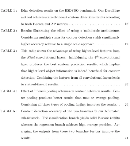
TABLE 1 : Edge detection results on the BSDS500 benchmark. Our DeepEdge

method achieves state-of-the-art contour detections results according

to both F-score and AP metrics. . . 18

TABLE 2 : Results illustrating the effect of using a multi-scale architecture.

Considering multiple scales for contour detection yields significantly

higher accuracy relative to a single scale approach. . . 19

TABLE 3 : This table shows the advantage of using higher-level features from

the KNet convolutional layers. Individually, the 4th _{convolutional}

layer produces the best contour prediction results, which implies

that higher-level object information is indeed beneficial for contour

detection. Combining the features from all convolutional layers leads

to state-of-the-art results. . . 20

TABLE 4 : Effect of different pooling schemes on contour detection results.

Cen-ter pooling produces betCen-ter results than max or average pooling.

Combining all three types of pooling further improves the results. . 20

TABLE 5 : Contour detection accuracy of the two branches in our bifurcated

sub-network. The classification branch yields solid F-score results

whereas the regression branch achieves high average precision.

Av-eraging the outputs from these two branches further improve the

(17)

TABLE 6 : Summary of results achieved by our proposed method (HfL) and

state-of-the-art methods (SotA). We provide results on four vision

tasks: Boundary Detection (BD), Semantic Boundary Labeling (SBL),

Semantic Segmentation (SS), and Object Proposal (OP). The

eval-uation metrics include ODS F-score for BD task, max F-score (MF)

and average precision (AP) for SBL task, per image intersection over

union (PI-IOU) for SS task, and max recall (MR) for OP task. Our

method produces better results in each of these tasks according to

these metrics. . . 25

TABLE 7 : Boundary detection results on BSDS500 benchmark. Upper half of

the table illustrates the results for “consensus” ground-truth

crite-rion while the lower half of the table depicts the results for “any”

ground-truth criterion. In both cases, our method outperforms all

prior methods according to both ODS (optimal dataset scale) and

OIS (optimal image scale) metrics. We also report the run-time of

our method (_‡ GPU time) in the FPS column (frames per second),

which shows that our algorithm is faster than prior approaches based

on deep learning [11, 12, 13, 1]. . . 31

TABLE 8 : Results of semantic boundary labeling on the SBD benchmark using

the Max F-score (MF) and Average Precision (AP) metrics. Our

method (HfL) outperforms Inverse Detectors [14] for all 20 categories

according to both metrics. Note that using the CRF output to label

the boundaries produces better results than using the outputs from

(18)

TABLE 9 : Semantic segmentation results on the SBD and VOC 2007 datasets.

We measure the results according to PP-IOU (per pixel) and PI-IOU

(per image) evaluation metrics. We denote the original

DeepLab-CRF system and our proposed modification as DeepLab-CRF and

DL-CRF+HfL, respectively. According to the PP-IOU metric, our

pro-posed features (DL-CRF+HfL) yield almost equivalent results as the

original DeepLab-CRF system. However, based on PI-IOU metric,

our proposed features improve the mean accuracy by 3% and 1.9%

on SBD and VOC 2007 datasets respectively. . . 37

TABLE 10 : Comparison of object proposal results. We compare the quality

of object proposals using Structured Edges [15] and HfL

bound-aries. We evaluate the performance for three different IOU values

and demonstrate that using HfL boundaries produces better results

for each evaluation metric and for each IOU value. . . 42

TABLE 11 : Boundary detection results on BSDS500 benchmark. Our proposed

method outperforms all prior algorithms according to all three

eval-uation metrics. . . 51

TABLE 12 : We compare semantic segmentation results when using a color-based

pixel affinity and our proposed boundary-based affinity. We note

that our proposed affinity improves the performance of all

globaliza-tion techniques. Note that all of the inference methods use thesame

FCN unary potentials. This suggests that for every method our

semantic boundary based affinity is more beneficial for semantic

(19)

TABLE 13 : Semantic segmentation results on the SBD dataset according to

PP-IOU (per pixel) and PI-PP-IOU (per image) evaluation metrics. We

use BNF-SB to denote the variant of our method that uses only

semantic boundary based affinities. Additionally, we use

BNF-SB-SM to indicate our method that uses boundary and softmax based

affinities. We observe that our proposed globalization method

out-performs other globalization techniques according to both metrics by

at least 0.3% and 1.3% respectively. Note that in this experiment,

all of the inference methods usethe same FCN unary potentials.

Additionally, for each method except Dense-CRF (it is challenging

to incorporate boundary based affinities into the Dense-CRF

frame-work) we use our boundary based affinities, since those lead to better

results. . . 60

TABLE 14 : Summary of recent semantic segmentation models. For each model,

we report whether it requires: (1) CRF post-processing, (2) complex

loss functions, or (3) recurrent layers. We also list the size of the

model (using the size of Caffe [16] models in MB). We note that

unlike prior methods, our RWN does not need post-processing, it

is implemented using standard layers and loss functions, and it also

has a compact model. . . 64

TABLE 15 : Semantic segmentation results on the SBD dataset according to the

per-pixel Intersection over Union evaluation metric. From the

re-sults, we observe that our proposed RWN consistently outperforms

(20)

TABLE 16 : Quantitative comparison between our RWN model and several

vari-ants of the DeepLab system that use a dense CRF or a

domain-transfer (DT) filter for post-processing. These results suggest that

our RWN acts as an effective globalization scheme, since it produces

results that are similar or even better than the results achieved by

post-processing the DeepLab outputs with a CRF or DT. . . 76

TABLE 17 : Quantitative comparison of spatial segmentation smoothness. We

extract the boundaries from the predicted segmentations and

evalu-ate them against ground truth object boundaries using max F-score

(MF) and average precision (AP) metrics. These results suggest that

RWN segmentations are spatially smoother than the DeepLab-CRF

segmentations across all baselines. . . 79

TABLE 18 : Scene labeling results on the Stanford Background and Sift-Flow

datasets measured according to the overall IOU evaluation metric.

We use a DeepLab-largeFOV network as base model, and show that

(21)

TABLE 19 : We use the ImageNet VID [17] dataset to compare our STSN to the

state-of-the-art FGFA [18] and D&T [19] methods. Note that SSN

refers to our static baseline, which is obtained by using only the

reference frame for output generation (no temporal info). Also note,

that D&T+ and STSN+ refer to D&T and STSN baselines with

temporal post-processing applied on top of the CNN outputs. Based

on these results, we first point out that unlike FGFA, our STSN does

not rely on the external optical flow data, and still yields higher mAP

(78.9 vs 78.8). Furthermore, when no temporal post-processing is

used, our STSN produces superior performance in comparison to the

D&T baseline (78.9 vs 75.8). Finally, we demonstrate that if we

use a simple Seq-NMS [20] temporal post-processing scheme on top

of our STSN predictions, we can further improve our results and

outperform all the other baselines. . . 94

TABLE 20 : Pose detection results on the PoseTrack dataset measured in mAP.

The first row reports the results of a single-frame baseline [21], which

won the ICCV17 PoseTrack challenge. In the second row, we present

the results of our method, which is based on the same exact model

as [21] but it istrainedon pairs of frames with our DiMoFs training

scheme (the testingis still done on individual frames). These results

indicate consistent performance gains for each body joint, and a

mean mAP improvement of 2.2%. . . 114

TABLE 21 : Keypoint tracking results on the PoseTrack dataset using

Multi-Object Tracking Accuracy (MOTA) metric. As our baseline, we use

the ICCV17 PoseTrack challenge winning method [21]. Our model

is trained using the same architecture as [21], but using our DiMoFs

(22)

TABLE 22 : We examine how various factors affect spatiotemporal action

local-ization performance on JHMDB. We observe that learning DiMoFs

discriminatively through detection outperforms the model with the

same architecture but that was not trained with DiMoFs scheme by

5.3% and 9.7% mAP for δ = 0, and δ = 10 respectively (compare

column 2 to 4, and 3 to 6). We also note that replacing DiMoFs

off-sets with optical flow yields 50.6% mAP, which is 3.8% worse than

using DiMoFs (column 5 vs 6). . . 118

TABLE 23 : Our results on Diving48 dataset. In the top half of the table, we show

that our system achieves 24.1% accuracy and outperforms 2D

meth-ods TSN [22] and TRN [23]. We also observe that even using the

initial cluster ID histograms as features produces solid results (i.e.

17.2% and 21.4%). Note that replacing DiMoFs with optical flow

reduces the accuracy by 2.6% (compared to our 21.4%). Our model

does not perform as well as the pre-trained R(2+1)D [24] baseline.

However, our pre-training is done on a much smaller dataset, and on

a more general pose detection task. Without Kinetics pre-training,

we outperform R(2+1)D [24] by a solid 2.7% margin. Finally, we

show that combining DiMoFs with pre-trained R(2+1)D [24]

im-proves the results, suggesting complementarity of the two methods. 119

(23)

TABLE 25 : The quantitative results for action-object detection task on our

first-person action-object RGBD dataset according to max F-score (MF)

and average precision (AP) metrics. All methods except GBVS were

trained on our dataset using a leave-one-out cross validation. The

result indicates that EgoNet has the strongest predictive power with

at least 2.9% (MF) and 5.3% (AP) gain over other methods. We also

include our human study results, which suggest that human subjects

achieve better action-object detection accuracy than the machines

across most activities from our dataset. . . 134

TABLE 26 : Quantitative results on GTEA Gaze+ dataset for an action-object

detection task. To test each model’s generalization ability on GTEA

Gaze+ dataset, we train each methodonlyon our first-person

action-object RGBD dataset. Based on the results, we observe that EgoNet

exhibits the strongest generalization power. . . 139

TABLE 27 : Quantitative results on Social Children Interaction dataset [25] for

the visual attention prediction task. The dataset contains 9

first-person videos of children performing activities such as playing cards

games, etc. We note that to test each method’s generalization ability,

none of the methods were trained on this dataset. We show that

EgoNet outperforms all the other methods on this dataset, which

indicates strong EgoNet’s generalization power. . . 141

TABLE 28 : The quantitative important object prediction results on the

first-person important object RGBD and GTEA Gaze+ datasets

accord-ing to the max F-score (MF) and average precision (AP) metrics.

Our results indicate that even without using important object labels

our VSN achieves similar or even better results than the supervised

(24)

TABLE 29 : The quantitative results for atomic basketball event detection on

our first-person basketball dataset according to max F-score (MF)

metric. These results show that our method 1) outperforms prior

first-person methods and 2) that each component plays a critical role

in our system. . . 172

TABLE 30 : The quantitative results for our basketball assessment task. We

evaluate our method on 250 labeled pairs of players, and predict,

which of the two players in a pair is better. We then compute the

accuracy as the fraction of correct predictions. We report the results

of various baselines in two settings: 1) using our predicted atomic

events, and 2) using ground truth atomic events. These results show

that 1) our model achieves best results, 2) that each of our proposed

components is important, and 3) that our system is pretty robust to

atomic event recognition errors. . . 174

TABLE 31 : We assess each method on two tasks: predicting a player’s future

motion (PFM), and capturing the goals of real players (CG). The

↑ and _↓ symbols next to a task indicate whether a higher or lower

number is better, respectively. Our method outperforms the

base-lines for both tasks, suggesting that we can generate sequences that

(1) are more similar to a true player’s motion and (2) capture the

goals of real players more accurately. We also note that removing a

goal verifier (“Ours w/o GV”) leads to a sharp decrease in

(25)

LIST OF ILLUSTRATIONS

FIGURE 1 : Egocentric images recorded using a GoPro camera attached to a

person’s head. The recorded first-person images capture almost

exactly what that person sees as he performs activities such as

cooking, or playing basketball. Such visual data allows us to infer

a person’s attention, his intentions, his skill level at a particular

activity, and even his decision making process in different situations. 3

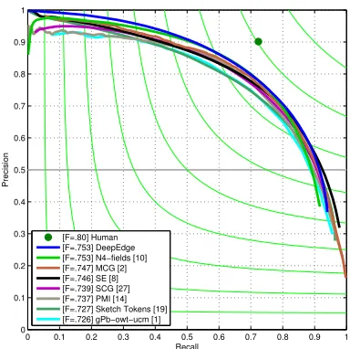
FIGURE 2 : Contour detection accuracy on the BSDS500 dataset. Our method

attains higher average precision compared to prior methods and

state-of-the-art F-score. At low recall, DeepEdge achieves nearly

100% precision. . . 7

FIGURE 3 : Visualization of multi-scale DeepEdge network architecture. To

extract candidate contour points, we run the Canny edge

detec-tor. Then, around each candidate point, we extract patches at four

different scales and simultaneously run them through the five

con-volutional layers of theKNet[26]. We connect these convolutional

layers to two separately-trained network branches. The first branch

is trained for classification, while the second branch is trained as

a regressor. At testing time, the scalar outputs from these two

sub-networks are averaged to produce the final score. . . 8

FIGURE 4 : Visualization of the activation values at the selected convolutional

filters of theKNet (filters are resized to the original image

dimen-sions). The filters in the second layer fire on oriented edges inside

the image. The third and fourth convolutional layers produce an

outline of the shape of the object. The fifth layer fires on the

(26)

FIGURE 5 : Detailed illustration of our proposed architecture in a single-scale

setting. First, an input patch, centered around the candidate point,

goes through five convolutional layers of theKNet. To extract

high-level features, at each convolutional layer we extract a small

sub-volume of the feature map around the center point, and perform

max,average, and center pooling on this sub-volume. The pooled

values feed a bifurcated sub-network. At testing time, the scalar

outputs computed from the branches of a bifurcated sub-networks

are averaged to produce a final contour prediction. . . 11

FIGURE 6 : A few samples of ground truth data illustrating the difference

be-tween the classification (first row) and the regression (second row)

objectives. The classification branch is trained to detect contours

that are marked by at least one of the human annotators.

Con-versely, the regression branch is optimized to the contour values

that depict the fraction of human annotators agreeing on the

con-tour. . . 13

FIGURE 7 : Qualitative results produced by our method. Notice how our method

learns to distinguish between strong and weak contours. For

in-stance, in the last row of predictions, contours corresponding to

zebra stripes are assigned much lower probabilities than contours

that correspond to the actual object boundaries separating the

ze-bras from the background. . . 17

FIGURE 8 : A visualization of selected convolutional feature maps from VGG

network (resized to the input image dimension). Because VGG

was optimized for an object classification task, it produces high

(27)

FIGURE 9 : An illustration of our architecture (best viewed in color). First we

extract a set of candidate contour points. Then we upsample the

image and feed it through 16 convolutional layers pretrained for

object classification. For each candidate point, we find its

corre-spondence in each of the feature maps and perform feature

inter-polation. This yields a 5504-dimensional feature vector for each

candidate point. We feed each of these vectors to two fully

con-nected layers and store the predictions to produce a final boundary

map. . . 27

FIGURE 10 : Qualitative results on the BSDS benchmark. The first column

of images represent input images. The second column illustrates

SE [15], while the third column depicts HfL boundaries. Notice

that SE boundaries are predicted with low confidence if there is no

significant change in color between the object and the background.

Instead, because our model is defined in terms of object-level

fea-tures, it can predict object boundaries with high confidence even if

there is no significant color variation in the scene. . . 32

FIGURE 11 : We train a linear regression model and visualize its weight

magni-tudes in order to understand which features are used most heavily

in the boundary prediction (this linear regression is used only for

the visualization purposes and not for the accuracy analysis). Note

how heavily weighted features lie in the deepest layers of the

net-work, i.e., the layers that are most closely associated with object

(28)

FIGURE 12 : A visualization of the predicted semantic boundary labels. Images

in the first column are input examples. Columns two and three

show semantic HfL boundaries of different object classes. Note that

even with multiple objects appearing simultaneously, our method

outputs precise semantic boundaries. . . 36

FIGURE 13 : In this figure, the first column depicts an input image while the

second and third columns illustrate two selected eigenvectors for

that image. The eigenvectors contain soft segmentation

informa-tion. Because HfL boundaries capture object-level boundaries, the

resulting eigenvectors primarily segment regions corresponding to

the objects. . . 39

FIGURE 14 : An illustration of the more challenging semantic segmentation

ex-amples. The first column depicts the predictions achieved by

DeepLab-CRF, while the second column illustrates the results after adding

our proposed features to the CRF framework. The last column

represents ground truth segmentations. Notice how our proposed

features render the predicted semantic segments more spatially

co-herent and overall more accurate. . . 41

FIGURE 15 : Examples illustrating shortcomings of prior semantic

segmenta-tion methods: the second column shows results obtained with a

FCN [27], while the third column shows the output of a

Dense-CRF applied to FCN predictions [28, 29]. Segments produced by

FCN are blob-like and are poorly localized around object

bound-aries. Dense-CRF produces spatially disjoint object segments due

to the use of a color-based pixel affinity function that is unable to

(29)

FIGURE 16 : We employ a semantic segmentation FCN [29] for two purposes:

1) to obtain semantic segmentation unaries for our global energy;

2) to compute object boundaries. Specifically, we define semantic

boundaries as a linear combination of these feature maps (with a

sigmoid function applied on top of the sum) and learn individual

weights corresponding to each convolutional feature map. We

inte-grate this boundary information in the form of pairwise potentials

(pixel affinities) for our energy model. . . 47

FIGURE 17 : An input image and convolutional feature maps corresponding to

the largest weight magnitude values. Intuitively these are the

fea-ture maps that contribute most heavily to the task of boundary

detection. . . 49

FIGURE 18 : A figure illustrating our boundary detection results. In the second

column, we visualize the raw probability output of our boundary

detector. In the third column, we present the final boundary maps

after non-maximum suppression. While most prior methods

pre-dict the boundaries where the sharpest change in color occurs, our

method captures semantic object-level boundaries, which we

sub-sequently use to aid semantic segmentation. . . 52

FIGURE 19 : A figure illustrating semantic segmentation results. Images in columns

two and three represent FCNsoftmax and Dense-CRF predictions,

respectively. Note that all methods use the same FCN unary

poten-tials. Additionally, observe that unlike FCN and Dense-CRF, our

methods predicts segmentation that are both well localized around

(30)

FIGURE 20 : Examples illustrating shortcomings of prior semantic segmentation

methods. Segments produced by FCNs are poorly localized around

object boundaries, while Dense-CRF produce spatially-disjoint

ob-ject segments. . . 63

FIGURE 21 : The architecture of our proposed Random Walk Network (RWN)

(best viewed in color). Our RWN consists of two branches: (1)

one branch devoted to the segmentation predictions , and (2)

an-other branch predicting pixel-level affinities. These two branches

are then merged via a novel random walk layer that encourages

spa-tially smooth segmentation predictions. The entire RWN is jointly

optimized end-to-end via a standard back-propagation algorithm. 65

FIGURE 22 : A figure illustrating the segmentation results of our RWN and the

DeepLab-v2 network. Note that RWN produced segmentations are

spatially smoother and produce less false positive predictions than

the DeepLab-v2 system. . . 73

FIGURE 23 : Comparison of segmentation results produced by our RWN

ver-sus the DeepLab-v2-CRF system. It can be noticed that, despite

not using any post-processing steps, our RWN predicts fine

ob-ject details (e.g., bike wheels or plane wings) more accurately than

DeepLab-v2-CRF, which fails to capture some these object parts. 75

FIGURE 24 : Localization error around the object boundaries within a trimap.

Compared to the DeepLab system (blue), our RWN (red) achieves

lower segmentation error around object boundaries for all trimap

widths. . . 77

FIGURE 25 : A figure illustrating how the probability predictions change as we

apply more random walk steps. Note that the RWN predictions

become more refined and better localized around the object

(31)

FIGURE 26 : IOU accuracy as a function of the number of random walk steps.

From this plot we observe that the segmentation accuracy keeps

improving as we apply more random walk steps and that it reaches

its peak when the random walk process converges. . . 81

FIGURE 27 : An illustration of the common challenges associated with object

detection in video. These include video defocus, motion blur,

oc-clusions and unusual poses. The bounding boxes denote the objects

that we want to detect in these examples. . . 84

FIGURE 28 : Our spatiotemporal sampling mechanism, which we use for video

object detection. Given the task of detecting objects in a particular

video frame (i.e., a reference frame), our goal is to incorporate

in-formation from a nearby frame of the same video (i.e., a supporting

frame). First, we extract features from both frames via a backbone

convolutional network (CNN). Next, we concatenate the features

from the reference and supporting frames, and feed them through

multiple deformable convolutional layers. The last of such layers

produces offsets that are used to sample informative features from

the supporting frame. Our spatiotemporal sampling scheme allows

us to produce accurate detections even if objects in the reference

(32)

FIGURE 29 : A figure illustrating some of our ablation experiments. Left: we

plot mAP as a function of the number of supporting frames used by

our STSN. From this plot, we notice that the video object detection

accuracy improves as we use more supporting frames. Right: To

understand the contribution of each of the supporting frames, we

plot the average weight magnitudes wt,t+k(p) for different values

of k. Here, p represents a point at the center of an object. From

this plot, we observe that the largest weights are associated with

the supporting frames that are near the reference frame. However,

note that even supporting frames that are further away from the

reference frame (e.g. k = 9) contribute quite substantially to the

final object detection predictions. . . 95

FIGURE 30 : An illustration of our spatiotemporal sampling scheme (zoom-in

for a better view). The green square indicates a point in the

ref-erence frame, for which we want to compute a new convolutional

output. The red square indicates the corresponding point predicted

by our STSN in a supporting frame. The yellow arrow illustrates

the estimated object motion. Although our model is trained

dis-criminatively for object detection and not for tracking or motion

estimation, our STSN learns to sample from the supporting frame

at locations that coincide almost perfectly with the same object.

This allows our method to perform accurate object detection even

(33)

FIGURE 31 : An illustration of using our spatiotemporal sampling scheme in

action. The green square indicates a fixed object location in the

reference frame. The red square depicts a location in a supporting

frame, from which relevant features are sampled. Even without

optical flow supervision, our STSN learns to track these objects

in video. In our supplementary material, we include more of such

examples in the video format. . . 98

FIGURE 32 : A figure illustrating object detection examples where our

spatiotem-poral sampling mechanism helps STSN to correct the mistakes

made by a static SSN baseline (please zoom-in to see the class

predictions and their probabilities). These mistakes typically

oc-cur due to occlusions, blurriness, etc. STSN fixes these errors by

using relevant object level information from supporting frames. In

Column 1 we illustrate the points in the supporting frame that

STSN considers relevant when computing the output for a point

denoted by the green square in Column 2. . . 101

FIGURE 33 : We extend modern detection models (e.g., Faster R-CNN) with

the ability to learn discriminative motion features (DiMoFs) from

RGB video data. We do so by training the detector on pairs of

time-separated frames, with the objective of predicting pose in one

frame using features from the other frame. This task forces the

net-work to learn motion “offsets” relating the two frames but that are

discriminatively optimized for detection. Our learned DiMoFs can

be used on a variety of applications: salient motion localization,

human motion estimation, improved pose detection and keypoint

tracking, spatiotemporal action localization, and fine-grained

(34)

FIGURE 34 : An illustration of our Discriminative Motion Feature (DiMoFs)

training procedure. Given Frame A and Frame B, which are

sepa-rated byδsteps in time, our goal is to detect pose in Frame A using

the features from Frame B. First, we extract multi-scale features

from both frames via a backbone CNN with shared parameters.

Then, at each scale, we compute the difference between feature

tensors A and B. From these tensor differences, offsets ∆pn are

predicted for each pixel locationpn. The predicted offsets are used

to re-sample feature tensor B. As a last step, the resampled feature

tensors from each scale are fed into a multi-scale detection head,

which is used to predict the pose in Frame A. Our scheme

opti-mizes end-to-end the DiMoFs network so that the feature tensors

re-sampled from Frame B maximize the pose detection accuracy in

(35)

FIGURE 35 : A figure with our DiMoFs visualizations. In the first two columns,

we visualize a pair of video frames that are used as input by our

model. The 3rd _{and 4}th _{columns depict 2 (out of 256) randomly}

selected DiMoFs channels visualized as a motion field. It can be

noticed that the DiMoFs capture primarily human motion, as they

have been optimized for pose detection. Different channels appear

to capture the motion of different body parts, thus performing a

sort of motion decomposition of discriminative regions in the video.

In the 5th _{column, we display the magnitudes of summed DiMoFs}

channels, which highlight salient human motion. Finally, the last

two columns illustrate the standard Farneback flow, and the human

motion predicted from our DiMoFs. To predict human motion we

train a linear classifier to regress the (x, y) displacement of each

joint from the offset maps. The color wheel, at the bottom right

corner encodes motion direction. . . 107

FIGURE 36 : We extend our DiMoFs architecture for spatiotemporal action

lo-calization. Given a pair of video frames–Frame A and Frame B—we

output for each person detected in Frame A, a bounding box and

an action class. Up until the RoI Align, our model operates in

the same way as for the pose detection task. Then, RoI Align is

applied on 1) the multi-scale FPN feature tensors from Frame A

(appearance), and 2) the multi-scale DiMoFs (motion). These RoI

features are then fed into separate MLPs, and the resulting

1024-dimensional features are used to predict a bounding box and an

(36)

FIGURE 37 : A high-level overview of our approach for learning fine-grained

ac-tion recogniac-tion features. Initially, we use our DiMoFs model to

ex-tract pose and DiMoFs features from a given pair of video frames.

We then accumulate these pose and DiMoFs features across the

entire Diving48 training set, and cluster them using a k-means

al-gorithm. The resulting cluster assignment IDs are then used as

pseudo ground truth labels to optimize our action recognition

fea-tures, as illustrated in Figure 36. . . 111

FIGURE 38 : Pose detection results on the PoseTrack dataset. Our model

pre-dicts pose in Frame A using features from a Frame B that is δ

time-steps away. Duringtraining, our model is optimized on frame

pairs with random time-gapsδ ∈ {−10, . . . ,10}. Here, we present

the results obtained by using different values of δ at inference

time. Asδ becomes large the motion between frames may become

substantial. Yet, the accuracy of our model drops gracefully asδ

deviates from 0. This confirms that our model estimates the human

motion between the two frames reliably. . . 113

FIGURE 39 : Our spatiotemporal action localization results on JHMDB dataset

as we vary the time-gapδseparating Frame B from Frame A during

inference. Based on these results, we observe that the performance

is lowest atδ = 0, which makes sense as there are no motion cues

to leverage. However, once δ gets larger, the accuracy increases

sharply indicating that the learned DiMoFs contain useful motion

(37)

FIGURE 40 : We predict action-objects from first-person RGBD images (best

viewed in color) where action-objects are defined as objects that

facilitate people’s conscious tactile (grabbing a food package) or

visual interactions (watching a TV). Left: a woman approaches a

shelf to pick up a food item (red). Right: The food (action-object)

is detected progressively as she approaches and reaches her hand

to pick it up. . . 123

FIGURE 41 : Our proposed EgoNet architecture (best viewed in color) takes as

input first-person RGB and DHG images, which encode 2D visual

appearance and 3D spatial cues respectively. The fully

convolu-tional RGB pathway then uses the visual appearance cues, while

the fully convolutional DHG pathway exploits 3D spatial

informa-tion to detect acinforma-tion-objects. The informainforma-tion from both

path-ways is combined via the joint pathway, which also implements the

first-person coordinate embedding, and then outputs a per-pixel

action-object probability map. . . 125

FIGURE 42 : The visualization of the fc7 activation values from the RGB and

DHG pathways. The RGB pathway has higher activations around

objects that stand out visually (e.g. a TV, a frying pan, a trash

bin), while the DHG pathway detects objects that are at a certain

distance and orientation relative to the person (e.g. a wine glass,

the gloves). . . 131

FIGURE 43 : Qualitative human study results averaged across 5 human subjects.

In many cases, third-person human subjects detect action-objects

correctly and consistently. However, some activities such as

shop-ping makes this task difficult even for a human observer since he

(38)

FIGURE 44 : An illustration of qualitative results on our dataset (the mirror

and the fry pan are the action-objects). Unlike other methods, our

EgoNet model correctly recognizes and localizes action-objects in

both instances. . . 137

FIGURE 45 : Qualitative results on GTEA Gaze+ dataset. EgoNet predicts

action-objects more accurately and with better localization

com-pared to DeepLab [29] based methods. . . 138

FIGURE 46 : Our results on Social Children Interaction Dataset. Strong EgoNet’s

generalization power allows it to predict action-objects in a novel

scenes, that contain previously unseen objects, and activities. . . . 140

FIGURE 47 : Given an unlabeled set of first-person images our goal is to find

all objects that are important to the camera wearer. Unlike most

prior methods, we do so without using ground truth importance

(39)

FIGURE 48 : We implement an interplay between the segmentation and

recog-nition agents via an alternating cross-pathway supervision scheme

inside our proposed Visual-Spatial Network (VSN). Our VSN

con-sists of the 1) visual (“what”) and 2) spatial (“where”) pathways,

which both act as recognition agents. In between these two

path-ways, the VSN uses an MCG projection scheme, which acts as a

segmentation agent. Then, given a set of unlabeled first-person

training images, we first guess “where” an important object is in the

first-person image and use an MCG projection scheme to propose

important object segmentation masks. These masks are then used

a supervisory signal to train a visual pathway such that it would

learn “what” an important object looks like. Then, in the V2S

round, the predictions from the visual pathway are passed through

the MCG projection, and transfered to the spatial pathway. The

spatial pathway then learns “where” an important object is in the

first-person image. Such an alternating cross-pathway supervision

scheme is repeated for several rounds. . . 146

FIGURE 49 : The qualitative important object predictions results. Despite not

using any importance labels during training, our VSN correctly

(40)

FIGURE 50 : A figure illustrating a qualitative important object prediction

com-parison between the visual and spatial pathways (best viewed in

color). Subfigure on the left illustrates instances where the spatial

pathway’s reliance on location features is beneficial: it detects small

and partially occluded important objects, which the visual

path-way fails to detect accurately. The Subfigure on the right shows

instances where the spatial pathway’s reliance on location features

leads to incorrect results: it falsely marks regions in the first-person

image as important objects just because they appear at a certain

location in the first-person image. In contrast, the visual pathway

correctly predicts important objects in those instances. . . 158

FIGURE 51 : Our results demonstrate that using a visual and a spatial pathway

(VSN) yields better important object detection accuracy than using

either two visual (VVN) or two spatial pathways (SSN). . . 159

FIGURE 52 : Our goal is to assess a basketball player’s performance from

un-scripted first-person basketball videos. During training, we learn

such a model from the pairs of weakly labeled first-person

bas-ketball videos. During testing, our model predicts a performance

measure customized to a particular evaluator from a given video.

Our model also discovers basketball events that contribute

(41)

FIGURE 53 : A detailed illustration of our basketball assessment prediction scheme.

Given a video segment from time interval [t, t+ 10], we first feed

it through a function fcrop, which zooms-in to the relevant parts

of a video. We then apply fevent to predict 4 atomic basketball

events from a zoomed-in video and a player’s (x, y) location on the

court. We then feed these predictions through a Gaussian mixture

functionfgm, which produces a highly non-linear visual

spatiotem-poral assessment feature. Finally, we use this feature to compute a

player’s assessment measure by multiplying it with linear weights

learned from the data, and with a predicted relevance indicator for

a given video segment. . . 170

FIGURE 54 : An illustration of of our training procedure to learn the linear

weights w that are used to assess a given basketball player’s

per-formance. As an input we take a pair of labeled first-person

bas-ketball videos with a label provided by a basbas-ketball expert

indicat-ing, which of the two players is better. Then, we compute visual

spatiotemporal basketball assessment features for all input video

segments, and use them to learn weightsw by minimizing our

for-mulated hinge loss function. . . 171

FIGURE 55 : We randomly select 4 pairs of basketball players, and visualize how

our assessment model evaluates each player over time. The red plot

denotes the better player in a pair, whereas the blue plot depicts

the worse player. The y-axis in the plot illustrates our predicted

performance measure for an event occurring at a specific time in a

(42)

FIGURE 56 : A visualization of basketball activities that we discovered by

man-ually inspecting Gaussian mixtures associated with the largest

bas-ketball assessment model weightsw. Each row in the figure depicts

a separate event, and the columns illustrate the time lapse of the

event (from left to right), We discover that the two most positive

Gaussian mixtures correspond to the events of a player making a

2 point and a 3 point shot respectively (the first two rows), while

the mixture with the most negative weight captures an event when

a player misses a 2 point shot (last row). . . 176

FIGURE 57 : A figure illustrating the events that contribute most positively (top

figure) and most negatively (bottom figure) to a player’s

perfor-mance measure according to our model. The red box illustrates

the location where our method zooms-in. Each row in the figure

depicts a separate event, and the columns illustrate the time lapse

of the event (from left to right). We note that among the detected

positive events our method recognizes events such as assists, made

layups, and made three pointers, whereas among the detected

neg-ative events, our method identifies events such as missed layups,

and missed jumpshots. . . 177

FIGURE 58 : Given a single first-person image from a one-on-one basketball

game, we aim to generate an egocentric basketball motion sequence

in the form of a 12D first-person camera configuration trajectory,

which encodes a player’s 3D location and 3D head orientation. In

this example, we visualize our generated motion sequence within a

(43)

FIGURE 59 : Our model takes a single first-person image as input and outputs

an egocentric basketball motion sequence in the form of a 12D

cam-era configuration trajectory, encoding a player’s 3D location and

3D head orientation throughout the sequence. First, we feed the

first-person image through our proposed future CNN to predict

an initial sequence of future 12D camera configurations. Then, we

use our proposed inverse synthesis procedure to synthesize a refined

camera configuration sequence that matches the configurations

pre-dicted by the future CNN, while also maximizing the output of the

goal verifier network. The goal verifier network is a fully-connected

network trained to verify that a given 12D camera configuration is

consistent with the final goals of real players. Finally, by

follow-ing the trajectory resultfollow-ing from the refined camera configuration

sequence, we obtain the complete 12D motion sequence. . . 185

FIGURE 60 : A figure illustrating the 3D locations of every camera configuration

from our dataset mapped on a 2D court (best viewed in color).

The blue points indicate the configurations from the beginning of

sequences, whereas the yellow points depict configurations from the

end of sequences. The diversity of real sequences in our dataset

(44)

FIGURE 61 : A figure illustrating some of our qualitative results. In the first

column, we depict an egocentric input image. In the second and

third columns, we visualize the activations of a Future CNN from

the res4a and res5c layers. Finally, in the last column, we present

our generated 2D motion trajectories. Based on the activations

of the Future CNN, we conclude that our CNN recognizes visual

cues in an egocentric image, which may be helpful for deciding

how to effectively navigate the court and reach the basket, or how

to get away from a defender. Furthermore, our generated motion

trajectories seem realistic, as they avoid colliding with the defender

and typically end near the basket, which reflects how most real

players would move. . . 194

FIGURE 62 : An illustration of the camera configurations generated by our

fu-ture CNN, which we visualize in a sparsely reconstructed 3D space

(best viewed in color). The red camera depicts the initial

cam-era configuration state, while the blue, magenta, green, and cyan

cameras correspond to the outputs from the 1st_,₂nd_,₃rd_{, and 4}th

branches of our future CNN, respectively. We note that our future

CNN is able to produce a diverse set of intermediate configurations,

which allows us to generate a wide array of different sequences at

a later step in our model. . . 195

FIGURE 63 : A visual illustration of our generated basketball sequences, in the

form of first-person images retrieved using nearest neighbor search.

We observe that our generated sequence is similar to a real

se-quence, suggesting that our model could be used for applications

(45)

FIGURE 64 : A figure comparing the final images of our generated sequences in

two settings: without and with using the goal verifier network.

We retrieve these images via nearest neighbor search. Note that

the images produced with a goal verifier “focus” on the basket, just

as real players would, thus capturing the goals of real players more

(46)

Part I

(47)

CHAPTER 1 : Problem Overview

Understanding the core attributes of human behavior such as attention, intent, or skill level

is crucial for many applications. Nevertheless, directly measuring them is difficult because

these attributes require understanding what that person is thinking in a particular situation.

Now, imagine a scenario where we could “tap” into a particular person’s visual system and

see exactly what that person sees as he progresses through his day (see Figure 1). Could we

then use such visual data to answer questions such as “what is that person paying attention

to?”, “what is he doing now?”, “what will he do next?”, “how good is he at a particular

activity?”.

For instance, take a look at the first image in row one of Figure 1. This image illustrates

almost exactly what a person sees during a particular activity. Just by looking at this

image, we can immediately tell a few things about the person behind the camera. First, we

know that he is in the kitchen, and thus, he is probably cooking. Furthermore, it also seems

that his attention is currently focused on the kitchen stove, and thus we could predict that

he might approach the kitchen stove next. Finally, from some of the objects in the scene

(i.e. a steak on the cutting board), we can even guess what kind of dish he is preparing.

Similarly consider the sequence of images in row two of Figure 1. Just by looking at these

images, we can easily tell that the person is currently playing basketball. However, there

are also many other details in these images that reveal more subtle cues about this person.

For instance, from his current position on the court, we can infer that he is the point guard

in his team. Furthermore, throughout the sequence, we observe that by calling a certain

play he outmaneuvers both of the defenders, which allows him to create an open three

point shot for himself. Not only does such an action signifies that this person has a good

decision making ability, but it also reveals that he is a skilled shooter as we observe his shot

(48)

time t time t+5 time t+10

Figure 1: Egocentric images recorded using a GoPro camera attached to a person’s head. The recorded first-person images capture almost exactly what that person sees as he per-forms activities such as cooking, or playing basketball. Such visual data allows us to infer a person’s attention, his intentions, his skill level at a particular activity, and even his decision making process in different situations.

Why would knowing any of these things be useful? Consider an application of building a

personal AI assistant inside one’s home. Suppose such a system had access to the visual

data of a person cooking a meal (row one of Figure 1). With the ability to infer that

person’s attention and his intentions, such a system could automatically control gadgets

such as the kitchen stove, order missing materials when needed, and assist this person in

a number of different ways. Similarly, having access to a particular person’s visual feed

during activities such as basketball (row two of Figure 1), would allow us to build novel

systems for player’s decision making analysis and their skill assessment. This would be

highly beneficial as nowadays these tasks are still performed by humans, making it a costly

and a time consuming process.

Inspired by these ideas, we aim to build visual perception models for inferring the core

attributes of human behavior such as attention, intention, and skill. We identify two key

(49)

terms of object-level cues– a representation that would allow us to understand the observed

environment better. Second, we need models that can infer the core behavioral attributes

from the visual data. We refer to these two challenges as “learning to see”, and “seeing to

learn” respectively.

We tackle the problem of “learning to see” by developing techniques that extract

object-level information directly from raw visual data. To do so, we first propose two top-down

edge detectors: DeepEdge [1] and HFL [2], which utilize high-level object features for a

low-level boundary detection process. We show that due to the semantic nature of our

boundaries we can also use these boundaries to aid a number of high-level vision tasks

such as semantic object segmentation or object detection. In addition, we also present two

effective object segmentation methods, Boundary Neural Fields (BNF) [3] and

Convolu-tional Random Walk Networks (RWN) [4], which successfully integrate low-level affinity

cues for improved semantic object segmentation performance. Furthermore, we introduce a

novel Spatiotemporal Sampling Network (STSN) architecture, which we use for video object

detection [5], and discriminative motion feature learning [6].

Afterwards, we transition to the problem of “seeing to learn”. To tackle this problem,

we leverage first-person GoPro cameras, which allow us to study the interplay between a

person’s visual attention and his actions. First, we propose a concept of action-objects–

the objects that capture person’s conscious visual (watching a TV) or tactile (taking a

cup) interactions. We then present EgoNet [7], a joint two-stream network that holistically

integrates visual appearance (RGB) and 3D spatial layout (depth and height) cues to predict

per-pixel likelihood of action-objects using a supervised learning objective. Next, to enable

unsupervised learning of action-objects, we introduce a Visual-Spatial Network (VSN) [8]

consisting of spatial (“where”) and visual (“what”) pathways, which are optimized using

our proposed alternating cross-pathway supervision scheme.

Finally, we describe several approaches for behavior understanding in a complex basketball

(50)

first-person videos in an unscripted five-on-five basketball game [9]. Next, we propose a

model that takes as input a single first-person image capturing exactly what a player sees,

and then predicts his future motion trajectory [10].

In the subsequent chapters, we will discuss each of these systems in more detail.

Fur-thermore, we will present experiments validating the effectiveness of each method at its

(51)

Part II

(52)

CHAPTER 1 : DeepEdge: A Multi-Scale Bifurcated Deep Network

for Top-Down Contour Detection

1.1. Introduction

0 0.1 0.2 0.3 0.4 0.5 0.6 0.7 0.8 0.9 1 0 0.1 0.2 0.3 0.4 0.5 0.6 0.7 0.8 0.9 1 Recall Precision [F=.80] Human [F=.753] DeepEdge [F=.753] N4−fields [10] [F=.747] MCG [2] [F=.746] SE [8] [F=.739] SCG [27] [F=.737] PMI [14] [F=.727] Sketch Tokens [19] [F=.726] gPb−owt−ucm [1]

Figure 2: Contour detection accuracy on the BSDS500 dataset. Our method attains higher average precision compared to prior methods and state-of-the-art F-score. At low recall, DeepEdge achieves nearly 100% precision. Contour detection is typically considered a

low-level problem, and used to aid

higher-level tasks such as object detection [30, 31,

32, 33]. However, it can be argued that

the tasks of detecting objects and

predict-ing contours are closely related. For

stance, given the contours we can easily

in-fer which objects are present in the image.

Conversely, if we are given exact locations

of the objects we could predict contours just

as easily. A commonly established pipeline

in computer vision starts with with

low-level contour prediction and then moves up

to higher-level object detection. However,

since we claim that these two tasks are mutually related, we propose to invert this process.

Instead of using contours as low-level cues for object detection, we want to use

object-specific information as high-level cues for contour detection. Thus, in a sense our scheme

can be viewed as a top-down approach where object-level cues inform the low-level contour

detection process.

In this work, we present a unified multi-scale deep learning approach that uses higher-level

object information to predict contours. Specifically, we present a front-to-end

convolu-tional architecture where contours are learned directly from raw pixels. Our proposed deep