K-Means Cluster Analysis Of Cities Based On Their Inter-Distances

IJEDR1704217

International Journal of Engineering Development and Research (

www.ijedr.org

)

1356

K-Means Cluster Analysis Of Cities Based On Their

Inter-Distances

Hari Prasad Duvvada1_{, G Durga Rama Naidu}2_{, V Divya Sri}3

1-M.Tech Structures Student, 2,3-Assistant Professor,

Department of Civil Engineering, Aditya Institute Of Technology & Management

________________________________________________________________________________________________________

Abstract— In this research investigation, the author performs K-Means Clustering of 104 cities in the state of former

Andhra Pradesh (in India) using the attribute of distance between them. This attribute of distance is of very much importance because cities that are very near to each other have usually good connectivity and consequently high population density and good development index. That is the Inter-Distance between any two cities, or rather the Cluster

number assignment can be used as an index for knowing their developmental stature as well.

Keywords— K-Means Algorithm, Latitude, Longitude

________________________________________________________________________________________________________

I. INTRODUCTION

In the following paragraphs of this Introduction section, the authors present some previous researchers work in the domain of K-Means Algorithm’s application with regards some attribute of cities.

Clustering cities based on their socio-economic development in long time period is an important issue and may be used in many ways, e.g., in strategic regional planning. In this research investigation [1], the authors continue their recent study where cumulative attribute for each year replaces nine other attributes, called ‘vector of dynamics’. In their previous paper some original ranking method was proposed. Using the same data set, here they try out some classical clustering models such as Minimum sum of squares and Harmonic means clustering. Results for the two last models are obtained using Variable neighborhood search based heuristics. A comparative study among old and new results on 120 Russian large cities are provided and analyzed.

Nowadays, cities consume more energy to fuel their day-to-day activities. With the rise of electrical devices we face more challenges associated with energy control and distribution. Apart from this, we also spend a lot of energy trying to either heating or cooling our homes. In [2], the author’s illustrate an architecture to extract, load, transform, mine and forecast Big Data. This technological architecture makes use of a dataset containing electricity and gas consumption of homes distributed within multiple USA cities and states. The main purpose of author’s work consists in delivering to citizens a new form of self-monitoring their electricity and gas consumption, by comparing them to other homes within their cluster or state and by forecasting future energy consumptions. Moreover, the architecture also delivers to energy providers and cities a smarter overview of the energy landscape. This work uses simulated data from United States of America along with Hadoop, WEKA and Tableau to store and process Big Data, to produce clusters and time series forecasts, and to visualize information, respectively. The results reveal that, using this architecture, it is possible to produce accurate clusters of homes based on their energy consumption and it is also possible to forecast future electricity consumptions with a small margin of error.

In [3] the authors aimed to evaluate the similarity between US cities by clustering them based on postings from the classifieds website Craigslist. Craigslist is a data source that could provide particular insight into the character of a city because the content is community-driven and contains unfiltered natural language. The clustering was performed agnostic to geographic location so as to determine a more nuanced indicator of similarity. Here, the authors report their methods for creating feature vectors from the raw posts and their results from subsequently clustering the cities. The authors experimented with features that considered the metadata, categorical distribution, as well as the natural language of posts. After generating feature vectors for each city, they applied two clustering algorithms, k-means and mean shift, and then compared their outputs. Clustering with kmeans produced fairly consistent, promising clusters, whereas clustering with mean shift did not produce any meaningful clusters. Their results from clustering could prove useful as an input to supervised learning problems that involve cities, or the clustering may be interesting as a qualitative metric in and of itself.

IJEDR1704217

International Journal of Engineering Development and Research (

www.ijedr.org

)

1357

In [5], the authors address the issue of how closely the fortunes of suburbs are tied to the fortunes of the central city. The authors develop housing price indices for most of the zip codes in California and use them in a clustering procedure to determine whether city and suburban housing markets naturally aggregate or move separately. The authors find that central cities tend to group with their suburbs, suggesting that the housing markets of cities and suburbs are closely linked.

In [6], the authors create a typology of cities based on indicators from the economic sector; characterize it with several other indicators of consumption and emissions and predict the typology of a random city through a decision tree. Available for this analysis were 298 global cities and 23 indicators that were processed through various clustering algorithms (K-Means, DBSCAN, EM and hierarchical) in order to obtain the typologies. These were then characterised in two ways. First using only the variables from the economical sector and second using the variables from population, economy, emissions and consumptions. This was done so one could construct typologies based on economic sectors and to avoid problems with the missing values in the second set of variables. With the typologies and characterisation done, the correlations between variables, with and without highlighting the typologies, were analysed and discussed. Finally the decision trees were constructed. The results will show: the existence of five typologies using K-Means clustering; a characterisation of the typologies based on 8 economical sector and 15 other variables; several important correlations between indicators; the relevancy of the typologies between indicators correlations and two decision trees that predict the city’s typology with good accuracy levels.

Crimes cause terror and cost our society dearly in several ways. Data mining can be used to model crime profiling. In [7], the authors look at use of clustering algorithm for a data mining approach to analyze the crimes patterns. The authors look at k-means clustering to aid in the process of crime profiling. The authors applied these techniques to primary crime data from Delhi police first information report (FIR) records. In this study, firstly the authors desire to estimate which type of crime is dominant in Delhi city, India. Accordingly crime is divided into three types heinous crime, non-heinous crime and special & local laws violation. Second estimation is to find which area categories are more sensitive towards, areas categories which are considered are slums, residential, commercial, VIP zones, travel points and markets. Third is to show distributions of each crime type in every area category.

In [8], the authors describe a method used for public finance analysis by the House Research Department to group Minnesota cities into classes with similar characteristics. These groupings are called “clusters.” This is the fourth grouping of cities for analysis purposes used by the House Research Department of Minnesota city, (USA) since the original groupings published in January 1988.

II. K-MEANS ALGORITHMOVERVIEW

K-Means Clustering Method

Clustering is the classification of objects into different groups, or more precisely, the partitioning of a data set into subsets (clusters), so that the data in each subset (ideally) share some common trait - often according to some defined distance measure. K- Means method falls in the category of Partitional Clustering.

Common Distance measures

Distance measure will determine how the similarity of two elements is calculated and it will influence the shape of the clusters. They include:

1. The Euclidean distance (also called 2-norm distance) is given by:

 





2 / 1 1 2

,













_





 n i i i

y

x

y

x

d

2. The Manhattan distance (also called taxicab norm or 1-norm) is given by:

 









n i i i

y

x

y

x

d

1

,

3. Minkowski Distance

 

n





p

i p i i

y

x

y

x

d

/ 1 1

,





















IJEDR1704217

International Journal of Engineering Development and Research (

www.ijedr.org

)

1358

The K-means algorithm is an algorithm to cluster

m

objects based on attributes into K partitions, where

K



m

.

It assumes that the object attributes form a vector space.

An algorithm for partitioning (or clustering) N data points into K disjoint subsets

S

_j containing data points so as to minimize the sum-of-squares criterion

2

1

 

 





K

j m S

j m

j

x

J



where

x

_m is a vector representing the the

m

th data point and



_jis the geometric centroid of the data points in

S

_j.

Simply speaking K-means clustering is an algorithm to classify or to group the objects based on attributes/features into K number of group. K is positive integer number.

The grouping is done by minimizing the sum of squares of distances between data and the corresponding cluster centroid.

How the K-Mean Clustering algorithm works?

Figure 1 - Flowchart showing the working of the K-Means Algorithm

Step 1: Begin with a decision on the value of K = number of clusters .

Step 2: Put any initial partition that classifies the data into K clusters. You may assign the training samples randomly, or systematically as the following: Take the first k training sample as single-element clusters

Assign each of the remaining (

m



K

) training sample to the cluster with the nearest centroid. After each assignment, recompute the centroid of the gaining cluster.

Step 3: Take each sample in sequence and compute its distance from the centroid of each of the clusters. If a sample is not currently in the cluster with the closest centroid, switch this sample to that cluster and update the centroid of the cluster gaining the new sample and the cluster losing the sample.

Step 4 . Repeat step 3 until convergence is achieved, that is until a pass through the training sample causes no new assignments.

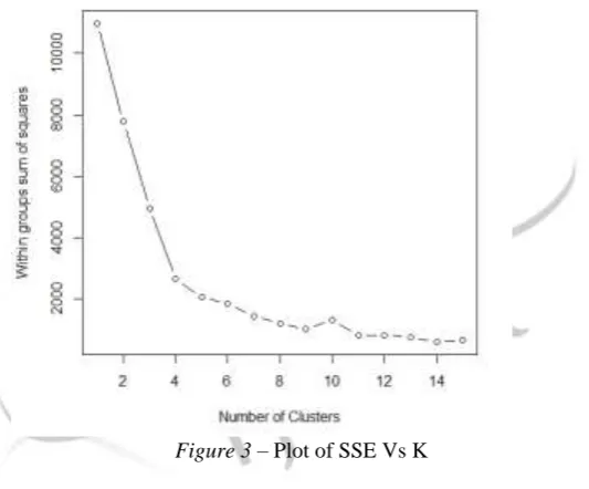
Choosing the right number (K) of Clusters – The Elbow Method

First of all, we compute the sum of squared error (SSE) for some values of K (for example 2, 4, 6, 8, etc.). The SSE is defined as the sum of the squared distance between each member of the cluster and its centroid. Mathematically, it is J _{as defined already.}

If we plot K against the SSE, we will see that the error decreases as K gets larger; this is because when the number of clusters increases, they should be smaller, so distortion is also smaller. The idea of the elbow method is to choose the K at which the SSE decreases abruptly. This produces an "elbow effect" in the graph of K against SSE.

III.K-MEANS CLUSTERINGAGORITHMRESULTS

Data Pre-Processing

IJEDR1704217

International Journal of Engineering Development and Research (

www.ijedr.org

)

1359

https://docs.google.com/spreadsheets/d/1WCxwGs2T-VrrMPDvwEvsGDxwapyfGogrWUzfwAaIKVQ/edit#gid=130852057

Latitudes & Longitudes Of Former Andhra Pradesh State In India

(1, 'Adilabad', '19.68 N', '78.53 E', 'Andhra Pradesh'), (2, 'Adoni', '15.63 N', '77.28 E', 'Andhra Pradesh'), (3, 'Alwal', '17.50 N', '78.54 E', 'Andhra Pradesh'), (4, 'Anakapalle', '17.69 N', '83.00 E', 'Andhra Pradesh'), (5, 'Anantapur', '14.70 N', '77.59 E', 'Andhra Pradesh'), (6, 'Bapatla', '15.91 N', '80.47 E', 'Andhra Pradesh'), (7, 'Belampalli', '19.06 N', '79.49 E', 'Andhra Pradesh'), (8, 'Bhimavaram', '16.55 N', '81.53 E', 'Andhra Pradesh'), (9, 'Bhongir', '17.52 N', '78.88 E', 'Andhra Pradesh'), (10, 'Bobbili', '18.57 N', '83.37 E', 'Andhra Pradesh'), (11, 'Bodhan', '18.66 N', '77.88 E', 'Andhra Pradesh'), (12, 'Chilakalurupet', '16.10 N', '80.16 E', 'Andhra Pradesh'), (13, 'Chinna Chawk', '14.47 N', '78.83 E', 'Andhra Pradesh'), (14, 'Chirala', '15.84 N', '80.35 E', 'Andhra Pradesh'), (15, 'Chittur', '13.22 N', '79.10 E', 'Andhra Pradesh'), (16, 'Cuddapah', '14.48 N', '78.81 E', 'Andhra Pradesh'), (17, 'Dharmavaram', '14.42 N', '77.71 E', 'Andhra Pradesh'), (18, 'Dhone', '15.42 N', '77.88 E', 'Andhra Pradesh'), (19, 'Eluru', '16.72 N', '81.11 E', 'Andhra Pradesh'),

IJEDR1704217

International Journal of Engineering Development and Research (

www.ijedr.org

)

1360

(61, 'Nuzvid', '16.78 N', '80.85 E', 'Andhra Pradesh'),

(62, 'Ongole', '15.50 N', '80.05 E', 'Andhra Pradesh'), (63, 'Palakollu', '16.52 N', '81.75 E', 'Andhra Pradesh'), (64, 'Palasa', '18.77 N', '84.42 E', 'Andhra Pradesh'), (65, 'Palwancha', '17.60 N', '80.68 E', 'Andhra Pradesh'), (66, 'Patancheru', '17.53 N', '78.27 E', 'Andhra Pradesh'), (67, 'Piduguralla', '16.48 N', '79.90 E', 'Andhra Pradesh'), (68, 'Ponnur', '16.07 N', '80.56 E', 'Andhra Pradesh'), (69, 'Proddatur', '14.73 N', '78.55 E', 'Andhra Pradesh'), (70, 'Qutubullapur', '17.43 N', '78.47 E', 'Andhra Pradesh'), (71, 'Rajamahendri', '17.02 N', '81.79 E', 'Andhra Pradesh'), (72, 'Rajampet', '14.18 N', '79.17 E', 'Andhra Pradesh'), (73, 'Rajendranagar', '17.29 N', '78.39 E', 'Andhra Pradesh'), (74, 'Ramachandrapuram', '17.56 N', '78.04 E', 'Andhra Pradesh'), (75, 'Ramagundam', '18.80 N', '79.45 E', 'Andhra Pradesh'), (76, 'Rayachoti', '14.05 N', '78.75 E', 'Andhra Pradesh'), (77, 'Rayadrug', '14.70 N', '76.87 E', 'Andhra Pradesh'), (78, 'Samalkot', '17.06 N', '82.18 E', 'Andhra Pradesh'), (79, 'Sangareddi', '17.63 N', '78.08 E', 'Andhra Pradesh'), (80, 'Sattenapalle', '16.40 N', '80.18 E', 'Andhra Pradesh'), (81, 'Serilungampalle', '17.48 N', '78.33 E', 'Andhra Pradesh'), (82, 'Siddipet', '18.11 N', '78.84 E', 'Andhra Pradesh'), (83, 'Sikandarabad', '17.47 N', '78.52 E', 'Andhra Pradesh'), (84, 'Sirsilla', '18.40 N', '78.81 E', 'Andhra Pradesh'), (85, 'Srikakulam', '18.30 N', '83.90 E', 'Andhra Pradesh'), (86, 'Srikalahasti', '13.76 N', '79.70 E', 'Andhra Pradesh'), (87, 'Suriapet', '17.15 N', '79.62 E', 'Andhra Pradesh'), (88, 'Tadepalle', '16.48 N', '80.60 E', 'Andhra Pradesh'), (89, 'Tadepallegudem', '16.82 N', '81.52 E', 'Andhra Pradesh'), (90, 'Tadpatri', '14.91 N', '78.00 E', 'Andhra Pradesh'), (91, 'Tandur', '17.25 N', '77.58 E', 'Andhra Pradesh'), (92, 'Tanuku', '16.75 N', '81.69 E', 'Andhra Pradesh'), (93, 'Tenali', '16.24 N', '80.65 E', 'Andhra Pradesh'), (94, 'Tirupati', '13.63 N', '79.41 E', 'Andhra Pradesh'), (95, 'Tuni', '17.35 N', '82.55 E', 'Andhra Pradesh'), (96, 'Uppal Kalan', '17.38 N', '78.55 E', 'Andhra Pradesh'), (97, 'Vijayawada', '16.52 N', '80.63 E', 'Andhra Pradesh'), (98, 'Vinukonda', '16.05 N', '79.75 E', 'Andhra Pradesh'), (99, 'Visakhapatnam', '17.73 N', '83.30 E', 'Andhra Pradesh'), (100, 'Vizianagaram', '18.12 N', '83.40 E', 'Andhra Pradesh'), (101, 'Vuyyuru', '16.37 N', '80.85 E', 'Andhra Pradesh'), (102, 'Wanparti', '16.37 N', '78.07 E', 'Andhra Pradesh'), (103, 'Warangal', '18.01 N', '79.58 E', 'Andhra Pradesh'), (104, 'Yemmiganur', '15.73 N', '77.48 E', 'Andhra Pradesh')

*Computation Of The Distance Between Two Pairs Of Latitude And Longitude

The website

https://www.movable-type.co.uk/scripts/latlong.html

allows one to calculate the distance between two pairs of latitude and longitude. Alternately, we have written an R program to compute the same using the formulae

Haversine

Formula

   











 













 



2

2

2 2 1

2









Sin

Cos

Cos

Sin

a

where











₂





₁



and











₂





₁





a

a



a

c



2

tan

2

,

1



Rc

d



where



_{is Latitude,}



_{is longitude, R is earth’s radius (mean radius = 6,371km); note that angles} need to be in radians to pass to trig functions!

Table 1- Formulae for Computing the distance between Latitudes and Longitudes of two different locations

IJEDR1704217

International Journal of Engineering Development and Research (

www.ijedr.org

)

1361

The K- Means Algorithm is used to find the Clusters among the 104 cities, based on the attribute of Distance between them. The program is detailed below:

rm(list=ls(all=TRUE)) getwd()

setwd("C:/Users/Desktop/HariPrasad ") #Consider mtacrs data of R-datasets data1<-read.csv("AllDistances.csv") mydata<-data1

mydata <- scale(mydata[,2:105]) # standardize variables summary(mydata[1])

str(data1$X)

###--- K- means Clustering ---### # K-Means Cluster Analysis with k = 5

fit <- kmeans(mydata, 5) # 5 cluster solution data1$cluster=fit$cluster

summary(fit)

#study the model and metrics

#With-in sum of squares in each cluster fit$withinss

sum(fit$withinss) fit$tot.withinss

#To check cluster number of each row in data fit$cluster

#Cluster Centers fit$centers # get cluster means

aggregate(mydata,by=list(fit$cluster), FUN=mean)

# append cluster label to the actual data frame mydata <- data.frame(mydata,fit$cluster) head(mydata)

# Determine number of clusters by considering the withinness measure wss <- 0

for (i in 1:15) {

wss[i] <- sum(kmeans(mydata,centers=i)$withinss) }

#Scree Plot plot(1:15, wss, type="b",

xlab="Number of Clusters",

ylab="Within groups sum of squares")

#Now we can perform any classification algorithm on the data to classify a future data point # For unseen data, we compute its distance from all the cluster centroids

# and assigns it to that cluster that is nearest to it test_datapoint <- mydata[1,]

closest.cluster <- function(x) {

cluster.dist <- apply(fit$centers, 1, function(y) sqrt(sum((x-y)^2))) print(cluster.dist)

return(which.min(cluster.dist)[1]) }

Results of the K-Means Clustering Algorithm

The aforedetailed K-Means Algorithm yielded the following results: It basically assigned Cluster Number based on their Inter-Distances values, for the thusly found optimal segregation as 5 Clusters.

IJEDR1704217

International Journal of Engineering Development and Research (

www.ijedr.org

)

1362

Figure 2 – The Summarized Output of the K-Means Algorithm

Finding The Optimal Number Of Clusters For Using The K-Means Algorithm

We implement the K-Means Algorithm for 1 to 15 number of clusters and we note that for the minimum error (within groups sum of squares) is at n=5. Hence, we choose n =5 as the Optimal Number of Clusters for using the K-Means Algorithm.

Figure 3 – Plot of SSE Vs K

IV.CONCLUSIONS

We conclude that the aforementioned 10,016 Inter-Distances for 104 cities cluster into 5 clusters, optimally speaking. AS the Inter Distance(s) between cities is a denominator of Development Index, we can say that the Development Index clusters into 5 Clusters or main categories.

ACKNOWLEDGMENT

The authors are grateful for the encouragement, advice and support offered by Prof G.T. Naidu, (HOD, Department Of Civil Engineering, Aditya Institute Of Technology & Management (AITAM), K. Kotthuru, Tekkali, Andhra Prdesh State India). The authors also are grateful to the former HOD Prof Ch. Kannam Naidu (AITAM). The authors also express their gratitude to Prof Murali Monangi, (formerly at AITAM).

REFERENCES

[1] B.S.Zhikharevich, O.V.Rusetskay, N.Mladenović, Clustering cities based on their development dynamics and Variable neigborhood search, Electronic

Notes in Discrete Mathematics, Volume 47, February 2015, Pages 213-220 https://doi.org/10.1016/j.endm.2014.11.028

[2] Carlos Costa and Maribel Yasmina Santos, Improving Cities Sustainability through the Use of Data Mining in a Context of Big City Data, Proceedings of

the World Congress on Engineering 2015, London, U.K., Vol I WCE 2015, July 1 - 3, 2015,

IJEDR1704217

International Journal of Engineering Development and Research (

www.ijedr.org

)

1363

[4] Shan Jiang, Joseph Ferreira, Marta C. González, Clustering daily patterns of human activities in the city, Data Min Knowl Disc (2012) 25:478–510 DOI

10.1007/s10618-012-0264-z

[5] William N. Goetzmann, Matthew Spiegel, Susan M. Wachter, Do Cities and Suburbs Cluster?, Cityscape: A Journal of Policy Development and Research,

Volume 3, Number 3, 1998 U.S. Department of Housing and Urban Development, Office of Policy Development and Research

[6] Bruno Miguel Fonseca de Oliveira, City Typologies: Classification and Characterization, Instituto Superior T´ecnico, Lisboa, Portugal October 2014

[7] Priyanka Gera , Rajan Vohra, City Crime Profiling Using Cluster Analysis, (IJCSIT) International Journal of Computer Science and Information

Technologies, Vol.5 (4), 2014, 5145-5148, ISSN:0975-9646

[8] Grouping Minnesota Cities Using Cluster Analysis’ Research Department Minnesota House of Representatives, September