Dynamic Model And Optimal Control Of A Snake Robot: TAROBOT 1

240 IJSTR©2015

________________________

 Tayfun Abut currently working as Research Assistant, Department of Mechanical Engineering in University of Mus Alparslan University, Turkey. E-mail:

[email protected]

Dynamic Model And Optimal Control Of A Snake

Robot: TAROBOT – 1

Tayfun Abut

Abstract: In this study, a model of snake robot is created and its dynamic modeling and control of a passive wheel planar is observed and studied. The main purpose of this work is to perform a corresponding movement in a stable condition with respect to the actual effect of environmental conditions. Serpanodial motion of the real snakes‘ is studied to determine the control of the robot. Holonomic constraints‘ of the system is taken into the consideration to obtain the robot‘s kinematics and dynamics equations. By using obtained dynamic equations, the model of the system is created in MATLAB/SIMULINK. The simulation studies showing performance of the system are performed by determining the control parameters of the system with Fuzzy and the Genetic Algorithm (GA) and controlling FUZZY PID, GA-PID and PID control. The system control parameters are determined by FUZZY PID, GA-PID and PID control the performance of the system by simulation studies have been performed. In addition, the dynamic motion simulations are carried out for obtaining data and experience before the experimental studies. Graphical results obtained are compared with the results of conventional PID control method applied to the system and the results are analyzed. Consequently, the computer simulations are shown that the suggested control methods are make the system control accomplished

Index Terms: Snake robot, Genetic Algorithm (GA), GA-PID, Dynamic equations, Fuzzy PID, PID

————————————————————

1

I

NTRODUCTION

Serpentine robots acting skills in almost any environment with high performance, long, thin and flexible to have a body, object manipulation skills and fine motor skills in harsh environments, has made it an interesting creature. In the literature, there are the robot studies about the snake robots in the different design and working space such as (2D, 3D) wheeled or crawler etc. and they are realizing many functions. Passive wheeled, planar robots constitute one of the main categories of the snake-like robots and they have been actively investigated. The first study about the snake robot was presented by Hirose in 1972[1]. The first snake robot had 2 meter height, 28 kg weight and it consisted of 20 joints. Also, it was equipped passive wheels. Later, the first snake robot was developed and called as R3 [2], wireless communication property. ACM-R3 had 1.8 meter height and 12 kg weight and it consisted of 20 joints. The robot mentioned above had two different rotation axis and its joints were connected with 90 perpendicular angle the each other. This type of connection made motion possible in 3D. Because, every connection point of this connection point of this connection had unique degree of freedom and this structure was standardize by simplifying of it. The later developed robot AmphiBott 2 [3], which is with passive wheel in 400 mm/s and it, had 770 mm height and 8 joints. Another snake robot study, Wheeko [4] had 10 joints and two actuator were used for every part of it.12 part passive wheel were bounded on the every joint and every part had two degree of freedom. Several studies were made by using different design and control methods [5-12]. Genetic algorithm is a method created by modeling on the evolution mechanism in the nature. Genetic algorithms are the research algorithms based on the natural selection and natural genetic mechanism, which may be summarized as "survival of the fittest in the natural system" suggested by Charles Darwin for the first time [13].

241

Figure 1: Photograph of the snake robot TAROBOT-1

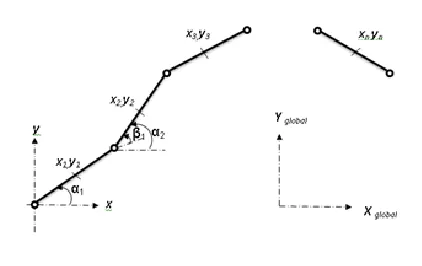
Figure 2: The module angle of the planar snake robot

Table1: Parameters for each of the joint

Symbol Description Units

Angle between joint i radian

Half the length of the

joint mm

Moment of inertia of the

joint kg.mm

2

m Mass of the joint kg

i

 Angle of the module radian

fx,i

Joint constraint force in x direction on joint i from

joint i+1.

N

fy,i

Joint constraint force in y direction on joint i from

joint i+1.

N

Table 2: Parameters for each of the joint

Symbol Description Units

fx,i-1

Joint constraint force in x direction on joint i from link

i-1.

N

fy,i

Joint constraint force in y direction on joint i from link

i-1.

N

ui

Actuator torque exerted on

link i from joint i+1. N.mm ui-1

Actuator torque exerted on

link i from joint i-1. N.mm fnx,i Friction force on joint in x

direction N

fty,i Friction force on joint in y

direction N

xi, yi

Global coordinates of the

center of mass of joint i. mm

Table 3: Parameters of robot

Symbol Description Units

kx

Global coordinates of the center of

mass of the snake robot mm ky

Global coordinates of the center of

mass of the snake robot mm xh

Coordinate in the direction of the

x-axis robot's head mm

yh

Coordinate in the direction of the

y-axis robot's head mm

2 Kinematic model of snake robot

The system is modeled by considering a simple planar snake robot model. The mass and moment of inertia are defined m,I respectively. Generalized coordinates of the system are q=[x1,y1, 1 … xn,yn,_n ]. Mass center of each joint are

represented by xi and yi.



i , _i states angle of the joint and

angle of the joint, respectively. As shown in figure 1 the length of each joint is 2l.

Figure 3: Planar snake model

1

i i i

    

(1)

In figure 2, i. the angle of the module is illustrates by i. Also,

i. the center of mass module is illustrates by xi and yi. In this study, position of robot and modules, which depend on the robot is determined by means of the right hand rule. In this context, motion axis matrix of the robot and the position of the robot head are illustrated by R and (xh, yh) respectively.

(2)

i



1,...v



(3)

The velocity expressions of gravity center of i. module are expressed by derivativing the position variable with respect to time variable by the following formula.

Ii

α

i

li

0

0

0 0 1

i i i i i Cos Sin Sin Cos R       _{ }        

 1 

1 1 1

2 cos cos

2 sin sin

i

i h j i

j i

i h j i

j

x x l l

y y l l

             





1 . . . . 1 1 . . . .

2 sin sin

2 cos cos

i

i h j j i i

j i

i

j j i

i h

x x l l

y y l l

242 IJSTR©2015

_i



_1,...v



(4) In this model there are two passive wheels on the center of gravity of each joint. Holonomic velocity constraints, which prevent these wheels to fall sideways, are calculated by following equation [15].

(5)

By simplifying after substituting equations 4 into eq. 5, next equation is obtained.

(6)

(7)

The equations expressed by FA and FB demonstrate the angle

of the joints and coordinates the head of the robot respectively.

3 Dynamic model of the planar snake robot

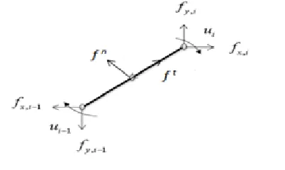
In obtaining dynamic equation of the system, L-E method is used not because L-E is systematic and easy but because L-E is used widely in robot dynamic equation of robot. Based upon to these equations, thanks to frictional forces acting on the module, the system is acted. The equations are derived by considering the moving of the robot on a flat surface. The equations of system are obtained like in [16], [17] and [18] which are widespread in literature. The system is exposed to externally applied forces during the movement, these forces may be categorized as those created by the environmental and system elements. Environmental forces are in the form of friction. Simple Coulomb friction model approach is used to achieve real target. Reaction forces are not shown in matrix form since L-E method will be used in the system. Each module is under the influence of moments, bond and friction forces. The forces and moments effecting to each joints are shown in Figure 4. Due to the rotation of the wheel, the friction force affects the system. This friction force devotes components of it. Reaction forces, from joint i-1. to joint i. , acts in x and y direction. Likewise, reaction forces from i + 1. joint acts to i. the joints. The size of the reaction force acting on the joint is the same but opposite direction.

Figure 4: The forces and moments acting on each module of

the snake robot

The kinetic energy of the system according to the general coordinates are obtained by utilizing the following equation.

(8)

( )

M  , 5 * 5 size is a positive definite symmetric matrix and at same time, it includes the inertia matrix of the system. Constants of the matrix are shown by M, L and J. There are variables of the matrix are only betas. Since robot works in the xy plane, the potential energy of the system is exposed to gravity acceleration in z direction. Z is always constant and V=z. The loss power of system is obtained by using the following the equation.

(9)

( )

N  is 5 * 5 is a matrix, which of variables are only



‘s and z is the constant of the N. Hence, when the Lagrange equatıons of the system is created, z=0 if L = T-V = T. In general Euler-Lagrange equation [18] is obtained by the following formula.

(10)

(11)

All environmental generalized forces are j

F

the forces, which are applied by F, except to the damping force due to rotation

.

p

_jis shown the state vector of the point, in whıch

F

_j is applied.



_i represents, except the generalized forces, the motor torque, whıch is required to follow the trajectory. Kinematic constraints are not included in Lagrange equations. Among the external forces, friction force is assumed as Coulomb friction and the falling of the system is prevented by it.

(12)

(13)

The centrifugal forces and Coriolis are shown in .

4 Numerical Simulation and Modeling

Serpanoid curve model is presented by Hirose [19]. This model is called serpentine model due to curve found in natural behaviors of snakes. In this model, motion similar to sinus is performed during body of snake. The relative angle between two successive modules is shown by



_i . φ , δ represents the angle of maximum deflection for each joint and the phase shift between any two adjacent joints respectively. The frequency and phase difference are illustrated by ω, ϑ respectively. Reference values are applied to the following formula. Figure 5 shows angle of the module of snake robot.

φ =π/6, δ = π/6, ϑ =0 and ω=π rad/s.

. .

sin cos 0

i _{i i i}

x  y  

1

. . . .

1

cos sin 2 cos( ) 0

i

h i

i i j i j

h

j

y x l l

     



      



. . 0 A B F F r  _       _{ }  

2 2 2

. . . . . 1 1 1 ( ) ( ) 2 2 T z

i _i i

T _m x y  J _ q M  q

 



2

1 . . .

1 1 1 ( ) 2 2 T z i

D c v q N q

 _{ }

 _{ } 

 



k k

i i i

d L L D

Q

dt q q q 

        _  _{ }     1 z j i j j i p Q F q    



i D q   ( )

i i i

f  m g sign v

 

..

.

,

.

.

M   _{ }  C_     _{ } N _{ }   Q

       

,

.

.

243 β i = φ sin(ω ⋅ t + (i −1) δ ) +ϑ i =1,2,3 [20] ( 14)

Figure 5: Angle of the module of snake robot

All tables and figures will be processed as images. You need to embed the images in the paper itself. Please don‘t send the images as separate files.

5 Control of snake robot

Modeling, control and numerical simulation of snake robot systems is carried out using the MATLAB software package. The MATLAB program of consists of a main program and two simulink program. Serpanodial motion is obtained by MATLAB simulink programs. This is the main program and subprograms are worked continuous simultaneously with each other in data exchange related. There are the initial values of the system in the main program, parameters of robot, dynamic equations and graphics commands for simulation. Simulink program is created by blocks and control parameters exist. Simulink program is a system consisting five inputs and five outputs. Serpanodial motion of snake robot is controlled by different control methods. The output signals of main program algorithm produced by PD, Genetic algorithm PID and Adaptive fuzzy PID control algorithms for the motors located in each joint of snake robot are appropriate torque values. The system is controlled by the obtained appropriate torque values. At the same time the effect of the controller on the system is shown. In the control algorithm, input of the system consists of e (the error) error and

e



(the rate of change of error) the exchange value of the error. Here, the error is the difference between the desired angle value and the output of the system. The outputs of the system are the appropriate torque values activating the motors, which minimizes the error and the change values in the error wıth respect to the time.

6 Adaptive Fuzzy PID

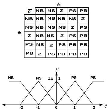
In this section, the control type of adaptive Fuzzy-PID is used by method of Mamdani‘s. The control system of the robot consists of an input and an output for each joint. Snake robot‘s control consists of five input and five output. All joints are used for the same rules table. Rule table is shown in Table 4. Control of the system is produced necessary control signals (



_i) which minimizes the error (

e

) and the change values in the error (

e



) with respect to the time.

Figure 6: The block structure of the control system and a

fuzzy controller

Simulink block structure of a fuzzy controller with the control system is shown in Figure 6. A FLC's (fuzzy logic controller) rule base consists of a group of IF-THEN rules usually have information about the system to be controlled experts obtained from individuals verbal expression. Rule base, FLC‘s is the most important part. A FLC rule base's considered the most important part. Because all other units and components is used for the realization of these rules in a fair and efficient manner. The rule base is created for the control of this system the following table 4 is consist of 25 rules, as shown.

Table 4: The rule base is generated for FLC

1

NB NS PS PB



ZE

0

-1 1 2

-2

e

Figure 7: The membership functions created for the input

values

e

1

NB NS PS PB



ZE

0

-1 1 2

-2

e



Figure 8: The membership functions created for the input

244 IJSTR©2015

1

NB NS PS PB



ZE

0

-2 2 4

-4



Figure 9: The membership functions created for the output

values



µ

ZE PB

NS

NB 1 PS

0.5

1

-0.5 0 0.5

-1

e. e,

Figure 10: The membership functions created for the

values

e

,

e



PM PVB

PS PB

1 0.2 0.4 0.6 0.8

µ ZE 1 0.5 Kp Ki Kd 0 0

Figure 11: The membership functions created for the values

kp, kd, ki

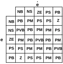
Table 5: The rule base is generated for Kp

NB NS ZE PVB PVB PB PB PB PM PM PS PS PS e NB NS ZE PS PB

PB PM PS

PM PM PS PS

PM PB

ZE

PS PM PVB

PM PB PB PVB

Kp

e.

Table 6: The rule base is generated for Kd

NB NS ZE PB PB PM PB PM PS PS Z Z PS e NB NS ZE PS PB

PM PS Z

PS PS Z Z

PS PM

ZE

Z PS PB

PS PM PM PB

Kd

e.

Table 7: The rule base is generated for Ki

NB NS PVB PB PVB PM PB PM PB PB Z PS PS NB ZE PS PB

PS PS Z

PB PM PM PS

PB PM

ZE

PM PM PVB

PS PS PM PB

e

NS

e

.

The degree of each membership function is a value between 0 and 1 consist of, triangular and gaussian membership functions are used. The graphics of the triangular membership functions for fuzzy control is shown in Figure 7, 8 and 9. Input values for the

e

and

e



{-2, -1, 0, 1, 2} is used that range. At the same time, the output value



for the fuzzy control {-4, -2, 0, 2, 4} is used in this range of values. In the above table shown the rule bases is created variables of the fuzzy is constructed as follows.

e

, (

e



),



= {Error, the error change, variable the control torque {NB (Negative Big), NS (Negative Small), ZE (Zero), PS (Positive Small), PB (Positive Big)}. FLC for the input values {-2, 2} are indicated range. All the input and output membership functions is taken as triangular type. In the adaptive fuzzy PID system are two inputs (

e

,

e



) and three outputs (kp, kd ki). PID coefficients are adapted with fuzzy and control of the system is realized. The graphs of Gaussian membership functions are shown in Figures 10 and 11. Input values for the

e

and

e



{-1, -0.5, 0, 0.5, 1} is used that range. At the same time, the output values kp-kd-ki for the adaptive fuzzy PID control {-4, -2, 0, 2, 4} is used in this range of values. The tables 5,6 and 7 are shown fuzzy variables in the rule bases, rules is created as below.

e

, (

e



)= { {Error, the error change, control, variable the control torque {NB (Negative Big), NM (Negative Medium), NS (Negative Small), Z (zero), PS (Positive Small), PM (Positive Medium), PB (Positive Big), PVB (Positive Largest),[-1, 1], µ}. Kp, Kd, Ki = {Control of parameters, {Z (zero), PS (Positive

Small), PM (Positive Medium), PB (Positive Big), PVB (Positive Largest), [0, 1], µ}. FLC for the input values {-1, 1} are indicated range. All of the input and output membership function is taken as the Gaussian type.

7 Genetic Algorithm

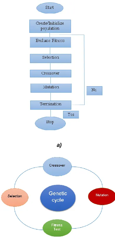
The followings are the steps used for implementation of the genetic algorithms.

1) Start:

Generally, start population (generation) is created from the random individuals (chromosomes).

2) Evaluate fitness:

Calculation of fitness values: Fitness values of each individual in the generation are calculated.

3) Selection:

Fitness values are selected from the generated population. 4) Crossover:

245 two solutions.

5) Mutation:

Information of the crossed chromosomes changes according to the mutation possibility. Mutation plays a secondary role as a decision maker in operation in GA's. The objective is to create new chromosomes by changing the places of one or more chromosomes.

6) Termination:

If result is satisfying, algorithm is terminated and the fittest chromosomes of the population presented as a solution, if not, following steps are carried out;

a)

Figure 12: a) Flow diagram of genetic algorithm b) Genetic

cycle

Fig. 12 shows flow diagram of genetic algorithm and genetic cycle. In brief, genetic cycle continues until finding an individual with the best fitness value. PID coefficient to be used for the control of snake robot has been optimized by using GA in this section. This optimization method can be adapted to the conditions by depending on the dynamic changes of the robot and developing the optimum PID controller parameters. Variable parameters of PID control have

been coded to solve the string structures of Kp, Ki, Kd. The population has been selected with random strings to create matching pool. Selected population strings will have mutation in the next step. The population that has been obtained forms the new population. Genetic algorithm parameters used in the simulation are showed in Table 8.

Table 8: Optimization parameters of genetic algorithm

8 Simulation with MATLAB-Simulink of the

system

Control of snake robot is realized with PD and Genetic algorithm PID and adaptive fuzzy PID (Proportional-Integral-Derivative). In the genetic algorithm PID the desired curve, in a short period of time necessary to achieve a stable structure to the reference value to be able to follow both the reference value, whether successful implementation of a control system in Figure 13 and Figure 14 are also seen. Genetic algorithm PID of control steady-state error is reduced both stable structure is reached reference is shown in Figure 13 and Figure 14.

9

R

ESULTS

Snake robot's dynamic model is realized. Serpanodial motion is obtained fairly successful results in modeling. The numerical simulation of the control system is made by using in Matlab / Simulink not only PID, genetic algorithm PID but also adaptive fuzzy PID control method and the results are presented in graphical forms. In this study, successful results are obtained about the control of snake robot by using different control methods. In order to avoid the disadvantage of PID control method, which is the reference input, the adaptive fuzzy PID and genetic algorithm PID control methods are used. Applied control method indicates the applicability of the control by following the reference value significantly. It is shown that adaptive fuzzy PID and genetic algorithm PID control methods are insensitive to both structural and non-structural uncertainty. MATLAB software program is used for the numerical solution. Responses are obtained and examined graphically. In this study, serpanodial motion is obtained.

10

C

ONCLUSION

246 IJSTR©2015

robot can be created in accordance with the other motions. In the light of this information for future work, focusing on

different designs and mechanisms are thought to provide high performance with a simpler mechanism design.

Figure 13: Results of numerical simulation for alpha 1

a)

b)

247

d)

Figure 14: Results of numerical simulation for a) alpha 2, b) alpha 3, c) alpha 4, d) alpha 5

R

EFERENCES

[1] S. Hirose, Biologically Inspired Robots: Snake-Like Locomotors and Manipulators. Oxford: Oxford University Press, 1993.

[2] M. Mori, S. Hirose, ‗‗Three-dimensional serpentine motion and lateral rolling by active cord mechanism ACM-R3,‘‘ in Proc. 2002 IEEE/RSJ Int. Conf. Intelligent Robots and Systems, 2002, pp. 829–834.

[3] Y. Umetani, ‗Mechanism and control of Serpentine movement,‘ International Biomechanism Symposium, 2004, pp 253-260.

[4] P. Liljebäck, Modelling, Development and Control of Snake robots Doctoral thesis at NTNU, 2011:70

[5] Aksel Andreas Transeth, Remco I. Leine, Christoph Glocker, Kristin Ytterstad Pettersen, P. Liljebäck, ―Snake robot obstacle-aided locomotion: modeling, simulations, and experiments‖, IEEE Transactions on Robotics, 2008, 24 (1): 88-104.

[6] G. Endo, K. Togawa and S. Hirose, Study on Self-contained and Terrain Adaptive Active Cord Mechanism, Proc. lEEE/RSI International Conference on Intelligent Robots and Systems, 1999, 1399-1405

[7] Abut T. , Soyguder S. ,Alli H. ―Bir Yilansi Robotun Dinamik Analizi ve Kontrolu‘‘ Ulusal Makine Teorisi ve Dinamiği Sempozyumu (UMTS) ,Atatürk Üniversitesi, 12-13 Eylül - Erzurum, 2013: 554-563

[8] Abut T. , Soyguder S. ,Alli H. ― Bir Yilansı Robotun Tasarimi ve Kinematik Analizi‘‘ Otomatik Kontrol Turk Milli Komitesi Ulusal Toplantisi TOK , Niğde Üniversitesi, 12-14 Ekim - Niğde, 2012: 580-584

[9] S. Hirose, Biologically Inspired Robots: Snake-Like Locomotors and Manipulators. Oxford: Oxford University Press, 1993.

[10]M. Mori, S. Hirose, ‗‗Three-dimensional serpentine motion and lateral rolling by active cord mechanism ACM-R3,‘‘ in Proc. 2002 IEEE/RSJ Int. Conf. Intelligent Robots and Systems, 2002, pp. 829–834.

[11]Y. Umetani, ‗Mechanism and control of Serpentine movement,‘ International Biomechanism Symposium, 2004, pp 253-260.

[12]P. Liljebäck, Modelling, Development and Control of Snake robots Doctoral thesis at NTNU, 2011:70

[13]Aksel Andreas Transeth, Remco I. Leine, Christoph Glocker, Kristin Ytterstad Pettersen, P. Liljebäck, ―Snake robot obstacle-aided locomotion: modeling, simulations, and experiments‖, IEEE Transactions on Robotics, 2008, 24 (1): 88-104.

[14]G. Endo, K. Togawa and S. Hirose, Study on Self-contained and Terrain Adaptive Active Cord Mechanism, Proc. lEEE/RSI International Conference on Intelligent Robots and Systems, 1999, 1399-1405

[15]Abut T. , Soyguder S. ,Alli H. ―Bir Yilansi Robotun Dinamik Analizi ve Kontrolu‘‘ Ulusal Makine Teorisi ve Dinamiği Sempozyumu (UMTS) ,Atatürk Üniversitesi, 12-13 Eylül - Erzurum, 2013: 554-563

[16]Abut T. , Soyguder S. ,Alli H. ― Bir Yilansı Robotun Tasarimi ve Kinematik Analizi‘‘ Otomatik Kontrol Turk Milli Komitesi Ulusal Toplantisi TOK , Niğde Üniversitesi, 12-14 Ekim - Niğde, 2012: 580-584

[17]Çetin N., Genetik Algoritma, Yüksek lisans tezi, Yıldız Teknik Üniversitesi Fen Bilimleri Enstitüsü, 2002 İstanbul.

[18]Kalyanmoy Deb, Optimization for Engineering Design Algorithm & Examples ,Indian Institute Of Technology Kanpur, Prentice Hall, 2005.

[19]C. Vlachos, D. Williams, and JB Gomm. Genetic approach to decentralised PI controller tuning for multivariable processes. In Control Theory and Applications, IEEE Proceedings-, volume 146, pages 58–64. IET, 1999.

248 IJSTR©2015

[21]T.O. Mahony, C J Downing and K Fatla, Genetic Algorithm for PID Parameter Optimization: Minimizing Error Criteria, Process Control and Instrumentation 2000 26-28 July 2000, University of Stracthclyde, pg 148-153.

[22]P. Prautsch, T. Mita Control and Analysis of the Gait of Snake Robots Proceedings of the 1999 lEEE International Conference on Control Applications Kohala Coast-Island of Hawai'i. Hawai'i, USA August 22-27, 1999

[23]W. Burdick, J. Radford and G. S. Chirikjian, ―A ―sidewinding‖ locomotion gait for hyper-redundant robots,‖ Vol. 9, No. 3, 1995. pp. 195 – 216.

[24]H. Date, Y. Hoshi, M. Sampei, and S. Nakaura, ―Locomotion control of a snake robot with constraint force attenuation,‖ in Proceedings of the American Control Conference, vol. 1, 2001, pp. 113–118.

[25]E.Kurtulmuş Locomotion and Control of a modular snake like robot 2010.

[26]Weisstein, Eric W., "Euler-Lagrange Differential Equation", MathWorld.

[27]S .Hirose, ―Biologically Inspired Robots: Snake –Like Locomotors and Manipulators,‖ Oxford University, 1993.