Analysis of the Bulk Queue Model with
Multiple Vacations, Delayed Service and
Closed Down Time
E. Rameshkumar1 and Benny Jacob P2
1
Department of Mathematics, CMS College of Science and Commerce (Autonomous), Coimbatore, Tamil Nadu, India
2
Department of Mathematics, Nehru College of Management, Coimbatore, Tamil Nadu, India
ABSTRACT
In this paper a / , /1 queueing system with multiple vacations, delayed service and closed down time is considered. If the queue size is less than after a service completion or after a vacation termination, the server goes for multiple vacation. After serving batches continuously even if sufficient number of customers are there in the queue, the server goes for a vacation with probability or resume service with probability
1 . After a vacation if the server finds at least customers waiting for the service he serves a batch size of
, customers, where . Various characteristics of the queueing system with numerical results are presented in this paper.
Key Words: Bulk arrival, bulk service, delayed service, multiple vacations, closed down time, steady state probability, performance measures, numerical computations.
Description of the Model
Server vacation models are useful for the systems in which the server wants to utilize the idle time for different purposes. Application of server vacation models can be found in manufacturing systems, designing of local area networks and data communication systems. This paper concentrates on a vacation system with multiple vacations, delayed service and setup time.
The objective of this chapter is to analyse a situation that exists in a pump manufacturing industry. A pump manufacturing industry manufactures different types of pumps, which require shafts of various dimensions. The partially finished pump shafts arrive at the copy turning center from the turning centre. The operator starts the copy turning process only if required batch quantity of shafts is available; because the operating cost may increase otherwise. After processing, if the number of available shafts is less than the minimum batch quantity, then the operator will start doing other work such as making the templates for copy turning, checking the components. Hence, the operator always shuts down the machine and removes the templates before taking up other works. When the operator returns from other work and finds that the shafts available are more than the maximum batch quantity, the server resumes the copy turning process, for which some amount of time is required to setup the template in the machine. Otherwise the operator will continue with other work until he finds required number of shafts. The above process can be modeled as / , /1 queueing system with multiple vacations, delayed service and setup times.
Various authors have analysed queueing problems of server vacations with several combinationsR. Arumuganathan and T. Judith Malliga analysed of a bulk queue with multiple vacations, delayed service and setup time[2]. A literature survey on queueing systems with server vacations can be found in Doshi [4]. Reddy et al. [6] have analysed a bulk queueing model and multiple vacations with setup time. They derived the expected number of customers in the queue at an arbitrary time epoch and obtained other measures. Recently, Ke [5] has analysed the optimal policy for / /1 queueing systems of different vacation types with startup time.
However, only a very few have done research on queueing systems with closedown time. In the analysis of a bulk queue with multiple vacations and closedown times R. Arumuganathan, S. Jeyakumar[1], considering closed down time. The performance measures are also obtained. It is observed that most of the studies on vacation queues concentrated only either on single server or single arrival with single vacation. Once the arrival occurs in bulk one can expect that the service can also be done in bulk. In practice, the server may requires some amount of time for closing the service after the service is completed and some amount of time for setup before the commencement of service..
The following points are addressed in this paper. multiple vacations concept is introduced with setup time with delayed service in a bulk queueing vacation model. Probability generating function (PGF) of queue length distributions at an arbitrary time epoch is obtained. A cost model to find optimal threshold value (minimum batch quantity) for the proposed queueing system has been developed. Important contribution is the study of cost model for a practical situation and how the results are useful in optimizing the cost.
The Queueing System / , /1 with Multiple Vacations, analyzed in this chapter assumes the following: 1. Units arrive in bulk at the system in a Poisson with mean rate λ and form a Queue.
2. The queue discipline is FIFO.
3. After completing a service if the queue length is less than ‘ ’ the server leaves for a vacation. When he returns if the queue length is still less than ‘a’ he leaves for another vacation and so on, until he finally finds at least ‘ ’ customers waiting for service.
4. After a service or vacation if the server finds at least ‘ ’ customers waiting for service, say , then he serves a batch of , customers, where .
The Mathematical Model
Let be a group size r.v of arrival, be the probability that ‘ ’ customers arrive in a batch and be the PGF of .
Let . , . and . be the cumulative distribution of service time, vacation times and closed down time respectively.
Let , and be the pdf’s of , and respectively.
, and denote the Laplace-Stieltjes transforms of , and respectively. denotes the remaining service time of a batch in service at an arbitrary time ,
and denote the remaining vacation time and closed-down time respectively of the server at time t.
and denote the number of customers in the queue and under service, respectively, at time .
We define such that
0 , when the server is , ;
1 is the no:of batches served upto time since the commencement of a busy period. We define such that
0 , 1 when the server is ,
when the server is .
The probabilities of the number of customers in the queue and service are defined as follows:
, , , , , 1 ;
, 1 ,
Which means that there are ‘ ’ customers in the queue, number of batches served upto and the server is busy with remaining service time .
, , , , , 0 ; 0,
and
, , , 1 ; 0
The following equations are obtained for Queueing System using Supplementary Variable Technique.
∆ , ∆ , 1 ∆ ∑ 0, ∆ (1)
∆ , ∆ , 1 ∆ ∑ , ∆ 0, ∆ ; 1 (2)
∆ , ∆ , 1 ∆ ∑ 0, 1 ∆ ;2 , 1 (3)
∆ , ∆ , 1 ∆ ∑ 0, ∆ ∑ , ∆ ; 1 1
(5)
∆ , ∆ , 1 ∆ ∑ , ∆ ; (6)
∆ , ∆ , 1 ∆ 0, ∆ (7)
∆ , ∆
, 1 ∆ 0, ∆ ∑ , ∆ ; 0; 1 1 (8)
∆ , ∆
, 1 ∆ 0, ∆ ∑ , ∆ ∑ 0, ∆ ; (9)
∆ , ∆ , 1 ∆ 0, ∆ ; 2 (10)
∆ , ∆ , 1 ∆ ∑ , ∆ 0, ∆ ; 1 1,
2 (11)
∆ , ∆ , 1 ∆ ∑ , ∆ ; , 2 (12)
Dividing the equations (1) to (11) by ∆ and letting the limit ∆ 0, the Steady State Queue Size Equations are obtained as,
∑ 0, (13)
∑ , ∆ 0, ; 1 (14)
∑ 0, 1 ; 2 , 1 (15)
∑ , 0, 1 ; 2 , 1 (16)
∑ 0 ∑ ; 1 1 (17)
∑ ; (18)
0, (19)
∑ , ∆ 0, ; 1 1 (20)
0, ∑ , ∑ 0, ; (21)
0, ; 2 (22)
∑ , 0, ; 1 1, 2 (23)
∑ , ; , 2 (24) The Laplace-Stieltjes transform of , and are defined respectively as follows:
∞
,
∞
,
Then the Laplace-Stieltjes transform of ′ , ′ and are defined respectively as follows:
′
∞
∞ ∞
0
′
∞
∞ ∞
0
∞
∞ ∞
0
0 ∑ 0 (25)
0 ∑ 0 ; 1 (26)
0 ∑ 0 1 ; 2 , 1 (27)
0 ∑ 0 1 ; 2 , 1 (28)
0 ∑ 0 ∑ ; 1 1 (29)
0 ∑ ; (30)
0 0 (31)
0 ∑ 0 ; 1 1 (32)
0 ∑ 0 ; (33)
0 0 ; 2 (34)
0 ∑ 0 ; 1 1, 2 (35)
0 ∑ ; , 2 (36)
Queue Size Distribution
Lee H. S has developed a new technique to find the steady state probability generating function of the number of customers in the system at an arbitrary time.
To apply this technique, the following probability generating function are defined.
, ∑ , , 0 ∑ 0 ;
, ∑ , , 0 ∑ 0 ; 1 , ∑∞ , , 0 ∑∞ 0
(37)
Multiplying the equations (25) by and (26) by 1 ; Summing up from i 0 ∞ and using (34), we have
0 0
∞
0
Using (37), we have
, , 0 , 0 ∑ 0 (38)
since
, ∑ , , 0 ∑ 0 and , 0 ∑∞ 0 .
Multiplying the equations (27) by and (28) by 1 ; Summing up from 0 ∞, we have
0 0 0 0 1
Using (37), we get
, , 0 ∑ 0 , 0 1 (39)
since
, ∑ and , 0 ∑ 0 ; 1
Multiplying the equations (29) by 0 1 and (30) by and summing up from
0 ∞, we have
where
∞ ∞ ∞ ∞
Using (37), we have
, , 0 , 0 ,
Hence
, , 0 ∑ ∑ 0 (40)
Multiplying the equations (31) by , (32) by 1 1 and (33) by ; Summing up from
0 ∞, we have
, , 0 0 0
Using (37), we have
, , 0 ∑ 0 ∑ 0 (41)
since
, ∑ , , ∑ and , 0 ∑ 0 ; 1.
Multiplying the equations (34) by , (35) by 1 1 and (36) by ; Summing up from
0 ∞, we have
0 0 ; 2
Using (37), we have
, , 0 ∑ 0 ; 2 (42) since
, ∑ and , 0 ∑ 0 ; 1. Substituting in equations (38) to (42), we have
, 0 , 0 ∑ 0 (43)
, 0 ∑ 0 , 0 1 (44)
, 0 ∑ ∑ 0 (45)
, 0 ∑ 0 ∑ 0 (46)
, 0 ∑ 0 ; 2 (47)
Using the expressions of , 0 , , 0 , , 0 , , 0 and , 0 from (43) to (47) respectively in (38) to (42), we have
Using (43) in (38), we have
, , 0 0
(48)
, 0 , 0 1
(49)
Using (45) in (40), we have
, 0
(50) Using (46) in (41), we have
, 0 0
(51) Using (47) in (42), we have
, 0
(52) Let be the PGF of the queue size at an arbitrary time epoch is the sum of PGF of queue size at service completion epoch and vacation completion epoch, then
, 0 , 0 , 0 (53) i.e.
, 0 , 0 , 0 , 0
∞
By substituting 0 in the equations (48) to (52), then the equation (53) becomes
, 0 0 ∑ 0 , 0 1
0 1
0 0 0 1
, 0 0 1
(54)
0 0 , 0
0 0 0 , 0 0
Let us define
∑ 0 ∑∞ 0 (55)
1 1 ∑ 0 0 1 ∑
(56)
Taking lim . This is of the form . So we have to apply L’ Hospitals rule. Note that
1
1
1
Differentiating the numerator of (56) w.r.t and letting the limit as 1, we have
1 1 0 0
1 0
Differentiating the denominator of equation (56) w.r.t and taking the limit as 1, we have
0
Again we have the form . So we have to apply L’ Hospital’s rule again and proceed.
2 1 1 2
Hence
0 0
Steady State Condition
The Probability Generating Function has to satisfy 1 1. In order to satisfy this condition apply L’ Hospitals rule and evaluation lim and equating the expression to 1, we have
0 0
Since and are probabilities, it follows that left hand side of the above expression must be positive. Thus
1 1 if and only if 0. If / , then 1 is the condition to be satisfied for the existence of steady state for the model under consideration.
Computational Aspects.
Eq. (53) has unknowns , , , , , , , , . The following two theorems are proven to express in terms of in such a way that the numerator has only constants. Now Eq. (53) gives the PGF of the number of customers involving only unknowns. By Rouche’s theorem of complex variables, it can be proved that has 1 zeros inside and one of the unit circle | | 1. Since is analytic within and on the unit circle, the numerator must vanish at these points, which gives equations with unknowns. These equations can be solved by any suitable numerical technique.
Theorem 1
, , 1, , 1,
(60)
also s and s are the probabilities of the i customers arrive during vacation time and closed down time
respectively.
Proof 1. Using , 0 i.e. Eqs.(42) and (43), we can express ∑ , 0 in terms of 0 1 . Hence Eq. (59) gives the PGF of the number of customers involving only unknowns
, , , , , , , .
Special case:
As a special case, it may noted that when closed down time is zero and 0 for 1,2, , then the PGF obtained in (59) reduces to the following form
1 1 ∑ 0 0 1 ∑
(61) which coincides with the result of Reddy et al. [7].
Performance Measure 1. Expected length of idle period
Let be the idle period random variable, then the expected length of idle period is given by
, where is the idle period due to multiple vacation process, is the expected closed down time.
Define a random variable U as
Solving for , we get
1 1 .
(62)
and are the probabilities of k customers arrive during vacation time and the probabilities of i customers being in the queue at a departure epoch respectively
From (48) we get
1 .
then (62) becomes
1 ∑ ∑ ,
(63) Therefore the expected length of idle period is obtained as
1 ∑ ∑ .
(64) 2. Expected length of busy period
Let B be the busy period random variable and let us define the random variable J as
0, if the server finds less than ‘ ’ customers after first service
1 if the server finds atleast ‘ ’ customers after first vacation Now
/ 0 0 / 1 1 ,
0 1 .
Solving for in the above, we get the expected length of busy period as
0 ∑ .
(65) 3. Expected queue length
The expected queue length at an arbitrary time epoch is obtained by differentiating at 1 and is given by
4 ∑ ∑ , 0 ∑
(66) Cost Model
Our queueing model has bulk service rule with single server. The customers have to wait if sufficient batch quantity is not available, in such case the server will be on vacation. By considering this situation of customers waiting and the effective utilization of the operator and the machine, it is essential to have an optimal threshold value for a batch quantity. We develop a cost model through which the total cost involved in the system can be minimized. We derive an expression for finding the total average cost with the following assumptions:
: Start up cost
: Holding cost per customer : Operating cost per unit time
: Reward per unit time due to vacation :setup cost per unit time
The total average cost per unit time is obtained as
E
where
Practical Application Numerical Example
The above queueing model is analysed numerically with the following assumptions: i. Service time distribution is -Erlang with 2.
ii. Batch size distribution of the arrival is geometric with the mean 2.
iii. Vacation and setup time are exponential with the parameter 10 and 8 respectively. iv. Service capacity with minimum 3 and maximum 4.
The zeros of the function on ( are using mathcad 8 professional and the simultaneous equations are solved. Results are presented for the service rate 1 and arrival rate ranging from 0.5 to 0.8, service rate 1.5 and arrival rate 1 to 1.4, service rate 2 and arrival rate from 1.5 to 1.8, service rate 2.5 and arrival rate ranging from 1.8 to 2.3 in the following tables.
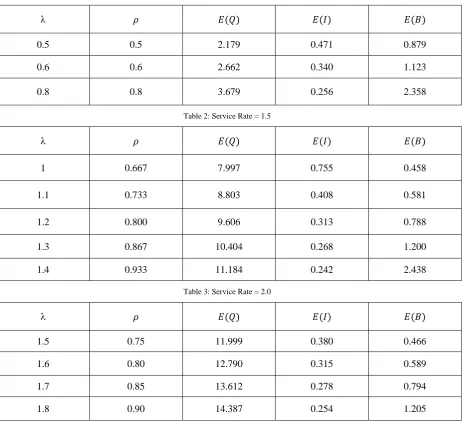
Table 1: Service Rate = 1.0
λ
0.5 0.5 2.179 0.471 0.879
0.6 0.6 2.662 0.340 1.123
0.8 0.8 3.679 0.256 2.358
Table 2: Service Rate = 1.5
λ
1 0.667 7.997 0.755 0.458
1.1 0.733 8.803 0.408 0.581
1.2 0.800 9.606 0.313 0.788
1.3 0.867 10.404 0.268 1.200
1.4 0.933 11.184 0.242 2.438
Table 3: Service Rate = 2.0
λ
1.5 0.75 11.999 0.380 0.466
1.6 0.80 12.790 0.315 0.589
1.7 0.85 13.612 0.278 0.794
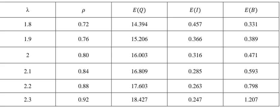
Table 4: Service Rate = 2.5
λ
1.8 0.72 14.394 0.457 0.331
1.9 0.76 15.206 0.366 0.389
2 0.80 16.003 0.316 0.471
2.1 0.84 16.809 0.285 0.593
2.2 0.88 17.603 0.263 0.798
2.3 0.92 18.427 0.247 1.207
From the above tables, following observations are made
i. As arrival rate ‘ ′ increases, the mean queue size increases.
ii. As queue size increases, expected length of idle period decreases and that of busy period increases. Conclusion
In this paper / , /1 queueing system with multiple vacations, delayed service and setup time the PGF of queue size at an arbitrary time epoch and various performance measure are obtained. Expression for total average cost is obtained. Cost model can also be analysed numerically for decision-making process. Further research can be carried out with this model with closed down time and N-policy.
References
[1] R. Arumuganathan, S. Jeyakumar, Analysis of a bulk queue with multiple vacations and closedown times, Int.J. Inform. Manage. Sci. 15 (1) (2004) 45-60.
[2] R. Arumuganathan, T. Judith Malliga, Analysis of a bulk queue with multiple vacations, delayed service and setup time.
[3] Arumuganathan, R., Bulk queuing models with server failures and multiple vacations, Ph.D. Thesis, Bharathiar University, Coimbatore, 1997.
[4] B.T. Doshi, Queueing systems with vacations: a survey, Queueing System (1986) 29-66.
[5] D.R. Cox, The analyses of non-Markovian stochastic processes by the inclusion of supplementary variables, Proc. Camb. Philos. Soc. 51 (1965) 433-441.
[6] G.V. Krishna Reddy, R. Nadarajan, R. Arumuganathan, Analysis of a bulk queue with N-policy multiple vacations and setup times, Comput. Oper. Res. 25 (11) (1998) 957-967.
[7] Ke Analysis of the optimal policy for / /1 queueing systems of different vacation types with startup time.
[8] H. Takagi, Queueing analysis: a foundation of performance evaluation, vol. I, Vacations and priority systems, part 1, North Holland, 1991. [9] H.S. Lee, Steady state probabilities for the server vacation model with group arrivals and under control operation policy, J. Korean OR/MS
Soc. 16 (1991) 36-48.
[10] H.W. Lee, S.S. Lee, J.O. Park, K.C. Chae, Analysis of the MX/G/1queue with N-policy and multiple vacations, J. Appl. Probab. 31(1994) 476-496.
[11] S.S. Lee, H.W. Lee, S.H. Yoon, K.C. Chae, Batch arrival queue with N-policy and single vacation, Comput. Oper. Res. 22 (2) (1995) 173-189.
[12] Marc, E., Herniter Programming in Matlab, Thomson Learning, Australia, 2001.
[13] K.C. Chae, H.W. Lee, MX/G/1vacation models with N-policy: heuristic interpretation of mean waiting time, J. Oper. Res. Soc. 46 (1995) 1014-1022.