Idealized models of the joint probability distribution of wind speeds

https://doi.org/10.5194/npg-25-335-2018 © Author(s) 2018. This work is distributed under the Creative Commons Attribution 4.0 License.

Idealized models of the joint probability

distribution of wind speeds

Adam H. Monahan

School of Earth and Ocean Sciences, University of Victoria, P.O. Box 3065 STN CSC, Victoria, BC, Canada, V8W 3V6 Correspondence:Adam H. Monahan ([email protected])

Received: 24 October 2017 – Discussion started: 2 November 2017

Revised: 6 February 2018 – Accepted: 26 March 2018 – Published: 2 May 2018

Abstract. The joint probability distribution of wind speeds at two separate locations in space or points in time com-pletely characterizes the statistical dependence of these two quantities, providing more information than linear measures such as correlation. In this study, we consider two models of the joint distribution of wind speeds obtained from ide-alized models of the dependence structure of the horizon-tal wind velocity components. The bivariate Rice distribu-tion follows from assuming that the wind components have Gaussian and isotropic fluctuations. The bivariate Weibull distribution arises from power law transformations of wind speeds corresponding to vector components with Gaussian, isotropic, mean-zero variability. Maximum likelihood esti-mates of these distributions are compared using wind speed data from the mid-troposphere, from different altitudes at the Cabauw tower in the Netherlands, and from scatterom-eter observations over the sea surface. While the bivariate Rice distribution is more flexible and can represent a broader class of dependence structures, the bivariate Weibull distribu-tion is mathematically simpler and may be more convenient in many applications. The complexity of the mathematical expressions obtained for the joint distributions suggests that the development of explicit functional forms for multivariate speed distributions from distributions of the components will not be practical for more complicated dependence structure or more than two speed variables.

1 Introduction

A fundamental issue in the characterization of atmospheric variability is that of dependence: how the state of one at-mospheric variable is related to that of another at a different

position in space, or point in time. The simplest measure of statistical dependence, the correlation coefficient, is a natu-ral measure for Gaussian-distributed quantities but does not fully characterize dependence for non-Gaussian variables. The most general representation of dependence between two or more quantities is their joint probability distribution. The joint probability distribution for a multivariate Gaussian is well known, and expressed in terms of the mean and co-variance matrix (e.g. Wilks, 2005; von Storch and Zwiers, 1999). No such general expressions for non-Gaussian multi-variate distributions exist. Copula theory (e.g. Schlözel and Friederichs, 2008) allows joint distributions to be constructed from specified marginal distributions. However, which cop-ula model to use for a given analysis is not generally known a priori and is usually determined empirically through a sta-tistical model selection exercise.

values at different spatial locations in the horizontal, depen-dence structures in the vertical (e.g. for vertical interpolation of wind speeds) or in time are also of interest. For example, an analysis in which the need for an explicit parametric form for the joint distribution of wind speeds at different altitudes has arisen is the hidden Markov model (HMM) analysis con-sidered in Monahan et al. (2015). In an HMM analysis of continuous variables, it is necessary to specify the paramet-ric form of the joint distribution within each hidden state. In Monahan et al. (2015), the joint distribution of wind speeds at 10 and 200 m and the potential temperature difference be-tween these altitudes was modelled as a multivariate Gaus-sian distribution, despite the fact that for at least the speeds this distribution cannot be strictly correct. This pragmatic modelling approximation was made because of the absence of a more appropriate parametric distribution for the quanti-ties being considered. The alternative approach of using the wind components at the two levels (for which the multivari-ate Gaussian model may be a better approximation) instead of the speeds directly has the downside of increasing the di-mensionality of the state vector from three to five, dramat-ically increasing the number of parameters to be estimated (with the covariance matrices in particular increasing from 9 to 25 elements) and reducing the statistical robustness of the results.

A number of previous studies have constructed univari-ate speed distributions starting from models for the joint dis-tribution of the horizontal components (e.g. Cakmur et al., 2004; Monahan, 2007; Drobinski et al., 2015). One use-ful benefit of this approach is that it allows the statistics of the speed and the components to be related to each other. The specific goal of the present study is to extend this ap-proach to bivariate distributions, constructing models of the joint probability distribution of wind speeds that are directly connected to the joint distributions of the horizontal com-ponents of the wind. As the following results will demon-strate, generalizing this approach to the bivariate speed dis-tribution results in rather complicated mathematical expres-sions. Expressions for multivariate distributions of more than two speeds will be even more complicated, and may not be analytically tractable. Through the analysis of the bivariate speed distribution, we will probe how far the development of closed-form, analytic expressions for parametric speed distri-butions based on distridistri-butions of components can practically be extended.

Both Weibull and Rice distributions have been used to model the univariate wind speed distribution (cf. Carta et al., 2009; Monahan, 2014; Drobinski et al., 2015), and models of multivariate distributions with Weibull or Ricean marginals have been developed (e.g. Crowder, 1989; Lu and Bhat-tacharyya, 1990; Kotz et al., 2000; Sagias and Karagianni-dis, 2005; Yacoub et al., 2005; Mendes and Yacoub, 2007; Villanueva et al., 2013). Much of this work has been done in the context of wireless communications (Sagias and Kara-giannidis, 2005; Yacoub et al., 2005; Mendes and Yacoub,

2007): the present study builds upon the results of these ear-lier analyses.

The two probability density functions (pdfs) we will con-sider, the bivariate Rice and Weibull distributions, both start with simple assumptions regarding the distributions of the wind components. The bivariate Rice distribution follows di-rectly from the assumption of Gaussian components with isotropic variance, but nonzero mean. In contrast, the bi-variate Weibull distribution is obtained from nonlinear trans-formations of the magnitudes of Gaussian, isotropic, mean-zero components. While the univariate Weibull distribution has been found to generally be a better fit to observed wind speeds than the univariate Rice distribution (particularly over the oceans, e.g. Monahan, 2006, 2007), the direct connec-tion of the Rice distribuconnec-tion to the distribuconnec-tion of the compo-nents (which the Weibull distribution does not have) is useful from a modelling and theoretical perspective (e.g. Cakmur et al., 2004; Monahan, 2012a; Culver and Monahan, 2013; Sun and Monahan, 2013; Drobinski et al., 2015). The six-parameter bivariate Rice distribution that we will consider is more flexible than the five-parameter bivariate Weibull dis-tribution, and able to model a broader range of dependence structures. Furthermore, it is directly connected to the uni-variate distributions and dependence structure of the wind components. However, the bivariate Weibull distribution is mathematically much simpler than the bivariate Rice distri-bution and easier to use in practice. Other flexible bivariate distributions for non-negative random variables exist, such as theα-µdistribution discussed in Yacoub (2007). Because the Weibull and Rice distributions are common models for the univariate wind speed distributions, this study will focus specifically on their bivariate generalizations.

The bivariate Rice and Weibull distributions are developed in Sect. 2, starting from discussion of the bivariate Rayleigh distribution (which is a limiting case of both of the other models). In this section, we repeat some of the formulae ob-tained by Sagias and Karagiannidis (2005), Yacoub et al. (2005), and Mendes and Yacoub (2007) for completeness and because of notational differences between this study and the earlier ones. In Sect. 3, the ability of these distributions to model wind speed data from the middle troposphere, and from the near-surface flow over land and the ocean, is con-sidered. Examples of dependence structures in both space (horizontally and vertically) and in time are considered. A discussion and conclusions are presented in Sect. 4.

2 Empirical models of the bivariate wind speed distribution

locations, two different points in time, or both). In particular, we assume that

1. the two orthogonal wind components are marginally Gaussian with isotropic and uncorrelated fluctuations:

ui vi

∼N

ui vi

,

σ_i2 0 0 σ_i2

i=1,2, (1)

2. and the cross-correlation matrix of the two vectors is

corr(u1,u2)=

corr(u1, u2) corr(u1, v2) corr(v1, u2) corr(v1, v2)

(2)

=

µ1 µ2 −µ2 µ1

=

ρcosψ ρsinψ −ρsinψ ρcosψ

,

where we have expressed the correlations in both Cartesian and polar coordinates: (µ1, µ2)= (ρcosψ, ρsinψ ), with 0≤ρ= µ2₁+µ2₂1/2_≤

1. This assumed correlation structure implies that the correlation matrix becomes diagonal when the vector

u2is rotated through the angle−ψ:

corr(u1, R(−ψ )u2)=

ρ 0

0 ρ

, (3)

where

R(−ψ )u2=

cosψ sinψ −sinψ cosψ

u2 v2

=

u2cosψ+v2sinψ −u2sinψ+v2cosψ

. (4)

The joint distribution of the horizontal components result-ing from these assumptions is

p(u1, u2, v1, v2)= 1 (2π )2_σ2

1σ 2

2(1−ρ2)

×exp − 1

2(1−ρ2₎

"

(u1−u1)2 σ₁2

+(v1−v1) 2 σ₁2

+(u2−u2) 2 σ₂2

+(v2−v2) 2 σ₂2

−2µ1[(u1−u1)(u2−u2)+(v1−v1)(v2−v2)] σ1σ2

−2µ2[(u1−u1) (v2−v2)−(v1−v1)(u2−u2)] σ1σ2

(5)

(Mendes and Yacoub, 2007).

Note that only considering the horizontal components of the wind vector implicitly restricts the resulting distributions to timescales sufficiently long that the vertical component of the wind contributes negligibly to the speed.

2.1 Bivariate Rayleigh distribution

The joint distributions of the speedswi=

q

u2_i +v_i2obtained from the pdf Eq. (5) when both vector wind components are mean-zero is the bivariate Rayleigh distribution (e.g. Bat-tjes, 1969). Transforming variables to wind speedwiand di-rectionθi=tan−1(vi/ui), the joint distribution (Eq. 5) with ui=vi =0,i=1,2, becomes

p(w1, w2, θ1, θ2)= w1w2 (2π )2_σ2

1σ22(1−ρ2)

exp − 1

2(1−ρ2₎

"

w₁2 σ₁2

+w 2 2 σ₂2

#!

×exp

_ρ

1−ρ2 w1w2

σ1σ2

cos(θ1−θ2+ψ )

. (6)

Integrating over the wind directions to obtain the marginal distribution for the wind speeds, we obtain

p(w1, w2)= w1w2

σ₁2σ₂2(1−ρ2₎exp − 1 2(1−ρ2₎

"

w2₁ σ₁2

+w 2 2 σ₂2

#!

Io

_ρ

1−ρ2 w1w2

σ1σ2

, (7)

where we have used the fact that 2π

Z

0

eαcosθcoskθdθ=2π Ik(α), (8)

whereIk(z)is the modified Bessel function of orderk. Note that the correlation angleψdrops out after integration over θ1andθ2. As a result, for the bivariate Rayleigh distribution, p(w1, w2)depends only on the three parameters(σ1, σ2, ρ).

For ρ=0, p(w1, w2) factors as the product of the marginal distributions ofw1andw2:

p(w₁, w₂)=

"

w₁ σ₁2exp −

w2₁ 2σ₁2

!# "

w₁ σ₁2exp −

w₁2 2σ₁2

!#

, (9)

and the wind speeds are independent. Asρ→1, we can use the asymptotic result

I0(x)∼ e x √

2π x (x

1) (10)

to show that

p(w1, w2)→ w1 σ₁2exp

−w 2 1 2σ₁2

!

δ

_w1

σ1 − w2

σ2

, (11)

0 0.5 0 1 2 3 w2 / σ2

0 1 2 3

0 0.5

ρ = 0

0 1 2 3

w 1/σ1

0 1 2 3 0 0.5 0 1 2 3 w2 / σ2

0 1 2 3

0 0.5

ρ = 0.5

0 1 2 3

w 1/σ1

0 1 2 3 0 0.5 0 1 2 3 w2 / σ2

0 1 2 3

0 0.5

ρ = 0.85

0 1 2 3

w 1/σ1

0 1 2 3

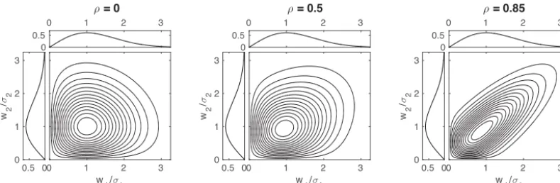
Figure 1.Example bivariate Rayleigh distributionsp(w1, w2)forρ=0,0.5, and 0.85, withw1andw2scaled respectively byσ1andσ2.

The upper and left subpanels show the marginal distributions ofw1andw2respectively. These marginal distributions are the same for all

three panels.

Moments of the bivariate Rayleigh distribution are given by

E

wm₁wn₂ = (12)

2m/22n/2σ₁mσ₂n0

1+m 2

0

1+n 2

2F1

−m 2,−

n 2,1;ρ

2_,

where2F1(α, β, γ;z)is the hypergeometric function (Grad-shteyn and Ryzhik, 2000). In particular, we have

mean(wi)=σi

r

π

2, (13)

var(wi)=2σi2

1−π 4

, (14)

corr(w1, w2)= π 4−π

2F1

−1 2,−

1 2,1;ρ

2_{−1. (15)}

Because 2F1(−1/2,−1/2,1;ρ2) is an increasing function ofρ2with2F1(−1/2,−1/2,1;0)=1, corr(w1, w2)must be non-negative for the bivariate Rayleigh distribution.

Plots ofp(w1, w2)for the three valuesρ=0, 0.5, and 0.85 are presented in Fig. 1, along with the marginal distributions ofw1andw2(which are the same for all three panels). The marginal distributions are positively skewed and the contours of the joint distributions are more tightly concentrated below and to the left of their peaks than elsewhere. As expected, the distributions become more tightly concentrated around the 1 : 1 line as the dependence parameterρincreases. 2.2 Bivariate Rice distribution

The assumptions leading to the bivariate Rayleigh distribu-tion are too restrictive to model observed wind speeds in most circumstances. A more general distribution results from as-suming that the wind components are Gaussian, isotropic, and uncorrelated, but with nonzero mean (Eq. 5).

Changing variables to wind speedwi and directionθi, the joint distribution becomes

p(w1, w2, θ1, θ2)=

w1w2

(2π )2_σ2 1σ

2 2(1−ρ2)

×exp − 1

2(1−ρ2₎

"

(w₁2+u2₁+v2₁) σ₁2 +

(w₂2+u2₂+v2₂) σ₂2

−2µ1(u1u2+v1v2)

σ1σ2

−2µ2(u1v2−v1u2)

σ1σ2

×exp

_w

1

σ1

a1cosθ1+

w2

σ2

a2cosθ2+

w1

σ1

b1sinθ1+

w2

σ2

b2sinθ2

+ 1

1−ρ2

w1w2

σ1σ2

(µ1cos(θ1−θ2)+µ2sin(θ1−θ2))

, (16) where

a1= 1 1−ρ2

_u1

σ1−µ1 u2 σ2−µ2

v2 σ2

= 1

1−ρ2

"

U1 σ1

cosφ1−ρU2 σ2

cos(φ2−ψ )

#

, (17)

b1= 1 1−ρ2

_v

1 σ1−µ1

v2 σ2+µ2

u2 σ2

= 1

1−ρ2

"

U1

σ1sinφ1−ρ

U2

σ2sin(φ2−ψ )

#

, (18)

a2= 1 1−ρ2

_u

2 σ2

−µ1u1 σ1

+µ2v1 σ1

= 1

1−ρ2

"

U2 σ2

cosφ2−ρU1 σ1

cos(φ1+ψ )

#

, (19)

b2= 1 1−ρ2

_v2

σ2−µ1 v1 σ1−µ2

u1 σ1

= 1

1−ρ2

"

U2 σ2

sinφ2−ρU1 σ1

sin(φ1+ψ )

#

, (20)

and where we have defined the magnitude and direction of the mean vector wind:

evalu-ate this integral, we make use of the result

1 (2π )2

2π Z 0 2π Z 0

exp [α1cosθ1+α2cosθ2+β1sinθ1+β2sinθ2

+γcos(θ1−θ2+ψ ) dθ1dθ2 =

∞

X

k=0 kcos

k

tan−1β1 α1−tan

−1β2 α2+ψ

×Ik

q

α₁2+β₁2

Ik

q

α₂2+β₂2

Ik(γ ), (22) where

k=

1 k=0

2 k6=0 (23)

and it is important that tan−1(b/a)be evaluated as the angle between the vector(a, b)and the vector(1,0)(that is, as the four-quadrant inverse tangent). Equation (22) follows from the Fourier series

eccosθ = ∞

X

k=0

kIk(c)coskθ (24)

along with repeated use of trigonometric identities and the integral Eq. (8).

Finally, we obtain the expression for the bivariate Rice dis-tribution (Mendes and Yacoub, 2007)

p(w1, w2)=

w1w2 σ₁2σ₂2(1−ρ2₎

×exp − 1

2(1−ρ2₎

"

(w₁2+u2₁+v2₁) σ₁2

+(w 2 2+u

2 2+v22) σ₂2 −2µ1(u1u2+v1v2)

σ1σ2 −

2µ2(u1v2−v1u2) σ1σ2

× ∞

X

k=0 kcos

k

tan−1b1 a1

−tan−1b2 a2

+tan−1µ2 µ1

×Ik

_w1

σ1

q

a₁2+b2₁

Ik

_w2

σ2

q

a₂2+b2₂

×Ik

_ρ

1−ρ2 w1w2

σ1σ2

. (25)

Expressed in terms of the magnitude and direction of the mean wind vectors,

p(w1, w2)=

w1w2 σ₁2σ₂2(1−ρ2₎

×exp − 1

2(1−ρ2₎

"

w2₁+U2₁

σ₁2 +w

2 2+U

2 2 σ₂2

−2ρU1U2cos(φ1−φ2+ψ ) σ1σ2

#!

× ∞

X

k=0

kcos(kν)Ik

w1 σ1

q

a2₁+b2₁

Ik w2 σ2 q

a2₂+b2₂

×Ik

_ρ

1−ρ2 w1w2

σ1σ2

, (26)

where

ν= (27)

tan−1 (1

−ρ2)U1U2

σ1σ2 sin(φ1−φ2+ψ ) (1+ρ2₎U1U2

σ1σ2 cos(φ1−φ2+ψ )−ρ

U2₁ σ₁2 +

U2₂ σ₂2

and

q

a2_i +b2_i = (28)

1 1−ρ2

"

U2_i

σ_i2 +ρ2U

2 3−i σ₃2_−i

−ρ2U1U2 σ1σ2

cos(φ1−φ2+ψ )

#

1 2 .

When numerically evaluating the bivariate Rice distribution, it is convenient to transform the infinite series in Eqs. (25) and (26) into an integral which is then approximated numer-ically (Appendix A).

Note that p(w1, w2)depends on the relative orientation of the mean wind vectors and the correlation angleψ only through the combinationφ1−φ2+ψ. Because of this symme-try, the quantitiesφ1−φ2andψcannot be determined indi-vidually from wind speed data alone. As a result,p(w1, w2) is determined by six parameters:(U1, σ1,U2, σ2, ρ, φ1−φ2+ ψ). For particular applications, it may be appropriate to fix either φ1−φ2 or ψ, allowing the other angle to be esti-mated from data. For example, when considering the tem-poral dependence structure of winds assumed to have sta-tionary statistics, it can be assumed that φ1−φ2=0. The bivariate Rice distribution also has the discrete symmetry that it is invariant under the transformationφ1−φ2+ψ→ −(φ1−φ2+ψ ). Note that these symmetries are in addition to the invariance of the distribution of components (Eq. 5) to the rotation of the coordinate systemθi→θi+1θ,i=1,2, under which the anglesφ1−φ2andψare individually invari-ant.

Integrating overw2to obtain the marginal distribution for w1we obtain the univariate Rice distribution

∞

Z

0

p(w1, w2)dw2=

w1

σ₁2exp − w2₁+U2₁

2σ₁2

!

I0

w1U1

σ₁2

!

, (29)

with mean and variance

mean(w1)=σ1

r

π 21F1 −

1 2,1,−

U2₁

2σ₁2

!

(30)

var(w1)=2σ₁2+U2₁−σ₁2π 21F

2 1 −

1 2,1,−

U2₁

2σ₁2

!

(with equivalent expressions forw2 obtained by integrating overw1), where1F1(α;β;z)is the confluent hypergeomet-ric function (Gradshteyn and Ryzhik, 2000). Equation (29) follows from Eq. (25) using the integral (Gradshteyn and Ryzhik, 2000)

∞

Z

0

xe−ax2Ik(bx)Ik(cx)dx=

1 2aexp

_b2_+c2 4a Ik _bc 2a , (32)

Neumann’s theorem (Watson, 1922) ∞

X

k=0

kIk(x)Ik(y)coskφ=I0

q

x2_+y2_+2xycosφ

, (33)

and the fact that cosν=

(1+ρ2)U1 σ1

U2

σ2 cos(φ1−φ2+ψ )−ρ

U2₁ σ₁2 +

U2₂ σ₂2

(1−ρ2₎2q_(a2

1+b21) a22+b22

. (34)

Note that each wind speed marginal distribution depends only on the magnitude of the mean wind vector, while the joint distribution also depends on the angle between the two mean wind vectors. Furthermore, asρ→0 only the first term contributes to the infinite series in Eq. (25), and the joint dis-tribution reduces to the product of the marginals.

The joint moments of the bivariate Rice distribution can be evaluated using the Taylor series expansion:

Ik

ρ 1−ρ2

w1w2 σ1σ2 = (35) ∞ X

j=0 1 j!(j+k)!

_ρ

2(1−ρ2₎

2j+k_w1

σ1

2j+k_w2

σ2

2j+k

,

which allows the double integral defining the moments to factorize as the products of individual integrals overw1and w2that can be evaluated using

∞

Z

0

xµe−αx2Ik(βx)dx= (36)

βk0(k+µ+1)/2 2k+1_α(µ+ν+1)/2_0(k+1)1F1

_k+µ+1

2 ;k+1; β2 4α

.

The resulting expression for the joint moments is Ewm₁wn₂ =2m/22n/2σ₁mσ₂n(1−ρ2)1+m/2+n/2

×exp − 1

2(1−ρ2₎

"

U2₁

σ₁2 +U

2 2 σ₂2

−2ρU1U2cos(φ1−φ2+ψ ) σ1σ2

#!

× ∞

X

l=0 l

X

k=0

"

kρ2l−kcos(kν)

0 l+m 2+1

0 l+n 2+1

l!(l−k)!(k!)2

×



(1−ρ2) q

(a₁2+b₁2)(a2₂+b2₂) 2





k

×₁F1 l+ m

2 +1;k+1;(1−ρ

2₎(a21+b21) 2

!

×1F1 l+n

2+1;k+1;(1−ρ

2₎(a22+b22) 2

!#

(37) (Mendes and Yacoub, 2007). When the mean vector winds are equal to zero, only thek=0 terms contribute to this ex-pression and Eq. (12) is recovered.

Defining the variablesVi=Ui/ √

2σi, the correlation co-efficient betweenw1andw2is given by

corr(w1, w2)= (38)

(1−ρ2₎2_exp

−V

2

1+V22−2V1V2cos(φ1−φ2+ψ ) (1−ρ2)

G(V1, V2, ρ, φ1−φ2+ψ )−π

4 1F1

−1 2;1; −V12

1F1

−1 2;1; −V22

h 1+V2

1−π4 1F1

−1 2;1; −V12

i12h

1+V2 2−π4 1F1

−1 2;1; −V22

i12

,

where

G(V1, V2, ρ, φ1−φ2+ψ )= ∞

X

l=0 l

X

k=0



kρ2l−kcos(kν)

02l+3 2

l!(l−k)!(k!)2

×



(1−ρ2) q

(a₁2+b₁2)(a2₂+b2₂) 2





k

×₁F1 l+ 3

2;k+1;(1−ρ 2₎(a

2 1+b

2 1) 2

!

×₁F1 l+ 3

2;k+1;(1−ρ

2₎(a22+b22) 2

!#

. (39)

The correlation coefficient corr(w1, w2) depends only on the four quantities(U1/σ1,U2/σ2, φ1−φ2+ψ, ρ). Monahan (2012b) considered the correlation structure of wind speeds using the approximation corr(w1, w2)'corr w2₁, w₂2. The assumed covariance structure of the wind components then results in the approximate expression:

corr(w1, w2)' ρ2+

u1u2 σ1σ2+

v1v2 σ1σ2

µ1+

u1v2 σ1σ2 −

v1u2 σ1σ2

µ2

s

1+u 2 1+v21

σ₁2 1+ u2

2+v22 σ₂2

=ρ

2₊U1U2

σ1σ2 cos(φ1−φ2+ψ ) ρ

s

1+U 2 1 σ₁2 1+

U2₂ σ₂2

-1 -0.5 0 0.5 1 ρ

-1 -0.5 0 0.5 1

Co

r

r

(

w1

,w

2

)

(U1/σ1,U2/σ2,φ1−φ2+ψ) = (3,2,0)

Approx. Bivar. rice

-1 -0.5 0 0.5 1

ρ -1

-0.5 0 0.5

1(U1/σ1,U2/σ2,φ1−φ2+ψ) = (0.5,4,0)

Approx. Bivar. rice

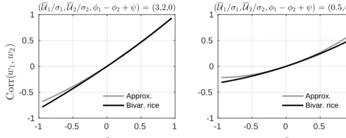
Figure 2. Comparison of the correlation coefficient corr(w1, w2)for bivariate Rice distributed variables (Eq. 38) with the approximate

expression Eq. (40) for the parameter values(U1/σ1,U2/σ2, φ1−φ2+ψ )=(3,2,0)and(0.5,4,0).

Plots of the correlation coefficient (Eq. 38) and the approx-imation (Eq. 40) as functions of ρ are shown in Fig. 2 for (U1/σ1,U2/σ2, φ1−φ2+ψ )= (3,2,0) and (1,5,0). Agreement between the exact and approximate values of the correlation coefficient is reasonably good in both cases, with the largest discrepancies generally occurring for larger absolute values of ρ. Note that negative wind speed correlation values are permitted by the bivariate Rice distribution.

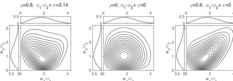
Examples of the joint Rice pdf (and the associated marginals) are presented in Fig. 3 for (U1, σ1,U2, σ2)= (6,4,2,5) and (ρ, φ1−φ2+ψ )=(0.85, π ), (0,0), and (0.85,0). By construction, the marginal distributions are the same in each panel. The distributions of both w1 andw2 are positively skewed, and take respective maxima at val-ues of about σ1 and just less than 2σ2. For the different values of the dependence parameter ρ, the joint tions have considerably different shapes. The joint distribu-tion for(ρ, φ1−φ2+ψ )=(0.8, π )describes (weakly) nega-tively correlated variables with a nonlinear dependence struc-ture evident in ridges of enhanced probability extending to the left and right upward from the probability maximum. For (ρ, φ1−φ2+ψ )=(0,0), probability contours are concen-trated towards smaller values ofw1andw2(as is the case for the marginal distributions). Finally,w1andw2are evidently positively correlated for(ρ, φ1−φ2+ψ )=(0.8,0), with a slight curvature in the shape of the distribution indicating the existence of some nonlinear dependence.

Although the bivariate Rice distribution differs from the bivariate Rayleigh distribution only by allowing for nonzero mean wind vector components, the resulting expressions for the joint pdf (Eq. 25) and the moments (Eq. 37) are much more complicated for the bivariate Rice than the bivariate Rayleigh. Furthermore, while the univariate Rice distribu-tion is a convenient model for the pdf of wind speed, ob-served winds show clear deviation from Ricean behaviour (e.g. Monahan, 2006, 2007). We will therefore consider an-other model of the bivariate wind speed distribution with Weibull marginals, which turns out to result in simpler

math-ematical expressions (at the cost of a more artificial deriva-tion than that of the bivariate Rice distribuderiva-tion).

2.3 Bivariate Weibull distribution

As in Sagias and Karagiannidis (2005) and Yacoub et al. (2005), we obtain the bivariate Weibull distribution from the bivariate Rayleigh distribution through separate power law transformations of w1 and w2. The pdf of a Weibull dis-tributed variable is

p(x)=b a

x

a

b−1

exp

−hx a

ib

, (41)

with moments E

xm =am01+m b

, (42)

whereaandbare denoted the scale and shape parameters re-spectively. The Rayleigh distribution is a special case of the Weibull distribution witha=

√

2σ andb=2. Weibull dis-tributed variables remain Weibull under a power law transfor-mation, with suitably modified scale and shape parameters: ifx is Weibull with scale parametera and shape parameter b,xkwill be Weibull with scale parameterak and shape pa-rameterb/ k. A joint wind speed distribution with Weibull marginal distributions can therefore be constructed from a joint Rayleigh distribution using the appropriate power law and scale transformations.

If we start with(x1, x2)as bivariate Rayleigh distributed withσi=1/

√

2, i=1,2, we obtain marginal Weibull dis-tributions with specified scale and shape parameters through the transformations

wi=aix_i2/bi. (43)

The joint pdfs transform as

p(w1, w2)=

∂x1w1 ∂x2w1 ∂x1w2 ∂x2w2

−1

0 0.5 0 1 2 3 w2 / σ2

0 2 4

0 0.5

ρ=0.8, φ₁-φ₂+ψ=3.14

0 2 4

w₁/σ₁

0 1 2 3 0 0.5 0 1 2 3 w2 / σ2

0 2 4

0 0.5

ρ=0,φ₁-φ₂+ψ=0

0 2 4

w₁/σ₁

0 1 2 3 0 0.5 0 1 2 3 w2 / σ2

0 2 4

0 0.5

ρ=0.8,φ₁-φ₂+ψ=0

0 2 4

w₁/σ₁

0 1 2 3

Figure 3.As in Fig. 1 for the bivariate Rice distribution with(U1, σ1,U2, σ2)=(6,4,2,5)and (ρ, φ1−φ2+ψ )=(0.8, π ), (0,0), and

(0.8,0).

and so we obtain the bivariate Weibull distribution

p(w1, w2)= 1 1−ρ2

b1b2 a1a2

_w1

a1

b1−1_w2

a2

b2−1

×exp − 1

(1−ρ2₎

" _w 1 a1 b1 + _w 2 a2

b2#!

×I0 2ρ (1−ρ2₎

_w

1 a1

b1/2_w

2 a2

b2/2!

. (45)

An analogous approach to constructing bivariate Weibull dis-tributions through nonlinear transformations of a bivariate Gaussian was followed in Villanueva et al. (2013); the re-sulting expressions are considerably more complicated than those considered here.

Evidently, p(w1, w2) factorizes into the product of the marginal distributions as ρ→0. As ρ→1, we can use Eq. (10) to make the approximation

p(w1, w2)' 1 1−ρ2

b1b2 a1a2

w1 a1

b1−1

w2 a2

b2−1

×exp − 1

(1−ρ2₎

" _w 1 a1 b1 + _w 2 a2

b2#!

× 4πρ

(1−ρ2₎

_w

1 a1

b1/2_w

2 a2

b2/2!−1/2

×exp 2ρ

(1−ρ2₎

_w1

a1

b1/2_w2

a2

b2/2!

' " b1 a1 _w1 a1

b1−1 exp −

_w1

a1

b1!#

× " b2 2a2 w1 a1

−b1/4

w2 a2

3b2/4−1#

×δ

_w

1 a1

b1/2 −

_w

2 a2

b2/2!

=p(w1)δ w2−a2

_w

1 a1

b1/b2!

, (46)

where the last equality follows from the fact that δ (f (x)−α)= 1

f0_(α)δ

x−f−1(α). (47)

As expected, w1 and w2 are completely dependent in the limit thatρ→1 (although they are not perfectly correlated ifb16=b2as the functional relationship

w2=a2

w1 a1

b1/b2

(48)

between the two variables will be nonlinear).

The relatively simple form of the bivariate Weibull distri-bution permits a relatively simple expression for the condi-tional distribution

p(w2|w1)=p(w1, w2) p(w1)

= ( b2 a2 _w 2 a2

b2−1 exp −

_w

2 a2

b2!)

×

(

1

1−ρ2exp − ρ2 1−ρ2

" _w1 a1 b1 + _w2 a2

b2#!

×I0 2ρ (1−ρ2₎

w1 a1

b1/2

w2 a2

b2/2!)

. (49)

The factor in the second set of braces characterizes how con-ditioning on the value ofw1changes the distribution ofw2 from its marginal distribution (and corresponds to a copula density; e.g. Schlözel and Friederichs, 2008). Note that for w1sufficiently large we can write

p(w2|w1)'

1

p

4πρ(1−ρ2₎ b2 a2

_w2

a2

3b2/4−1_w1

a1

×exp



−

1 1−ρ2

"

ρ

_w1

a1

b1/2 −

_w2

a2

b2/2#2



. (50)

Forρ not too close to zero, the conditional distribution for large w1 is concentrated around the nonlinear regression curve

w2 a2

b2 =ρ2

w1 a1

b1

. (51)

Computing the moments, we obtain E

wm₁wn₂ = (52)

a₁man₂0

1+m b1

0

1+ n b2

2F1

−m b1,−

n b2,1;ρ

2_.

(Sagias and Karagiannidis, 2005; Yacoub et al., 2005). The correlation coefficient is then given by

corr(w1, w2)= (53)

01+ 1

b1

01+ 1

b2

h

2F1

−1

b1,−

1 b2,1;ρ

2₋₁i r

h

0

1+_b2 1

−02₁₊ 1 b₁

i h

0

1+_b2 2

−02₁₊ 1 b₂

i

.

For b1, b2>1 (the relevant range of shape parameters for wind speeds), 2F1(−1/b1,−1/b2,1;ρ2) is an increasing function ofρ2with2F1(−1/b1,−1/b2,1;0)=1. Therefore, the bivariate Weibull distribution is unable to represent situ-ations in which the wind speeds are negatively correlated.

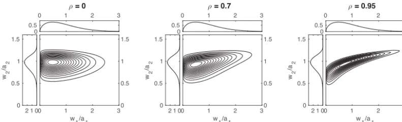
Examples of the bivariate Weibull distribution for (a1, b1, a2, b2)=(4,1.5,5,7)and values of ρ=0,0.7, and 0.95 are shown in Fig. 4. Again, the marginal distributions in all three cases are the same by construction. The distribu-tion ofw1is positively skewed with a maximum near a value ofw1=0.5a1, while that ofw2is negatively skewed with a maximum nearw2=a2. Forρ=0 the joint distribution is simply the product of the marginals. Asρincreases,w1and w2become positively correlated - although the correlation is weak even forρ=0.7 for this set of parameter values. At the value ofρ=0.95, while the correlation of the two variables is only moderate, a strong nonlinear dependence is evident in the concentration of the distribution around the curve given by Eq. (48).

3 Fits of bivariate Rice and Weibull distributions to observed wind speeds

Many wind datasets from different locations are available, and it is impracticable to consider joint distributions of wind speeds from even a small fraction of these. In this section, we will consider examples of the joint distribution of wind speeds using data from a representative range of settings. Bi-variate distributions of wind speeds at both different loca-tions in space and different points in time will be considered.

The sampling of the wind speeds considered will be tem-poral (that is, individual samples will correspond to a spe-cific time for spatial joint pdfs and a spespe-cific pair of times for temporal joint pdfs). Best-fit values of the parameters of the bivariate Weibull and Rice distributions we present were obtained numerically as maximum likelihood estimates (Ta-ble 1), withφ1−φ2set to zero. Goodness-of-fit of the dis-tributions was assessed using a statistical test described in Appendix B. In order to distinguish how well the paramet-ric joint distributions model the marginal distributions from how well they represent dependence between variables, the goodness-of-fit analyses were repeated for each pair of time series with the values of one of the pair shuffled in time. This shuffling destroys the dependence structure without affecting the distributions of the marginals. Use of a bivariate analysis rather than separate univariate goodness-of-fit tests for the marginals allows direct comparisons ofp-values, as exactly the same test is used for the original and shuffled data. 3.1 Wind speeds at 500 hPa

We first consider the joint distribution of 00Z December, January, and February 500 hPa wind speeds from 1979 to 2014. These data were taken from the European Centre for Medium-Range Weather Forecasts (ECMWF) ERA-Interim Reanalysis (Dee et al., 2011), subsampled to every sec-ond day to minimize the effect of serial dependence on the goodness-of-fit test (Monahan, 2012b). The wind speed data were computed as the magnitude of zonal and meridional components.

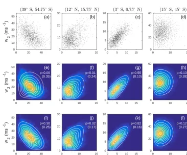
The joint distributions of wind speeds at four pairs of lat-itudes along 216◦_{W are presented in Fig. 5. A moderately} strong negative correlation (r= −0.55) is evident between wind speeds at (39◦S, 216◦W) and (54.75◦S, 216◦W) (Fig. 5a). Because it is unable to model a negative corre-lation between wind speeds, the best-fit bivariate Weibull pdf differs substantially from the distribution of the observed winds (Fig. 5e). The goodness-of-fit test correspondingly re-jects the null hypothesis that the observations are drawn from this distribution(p=0). In contrast, the bivariate Rice dis-tribution provides a reasonable model of the joint distribu-tion of wind speeds at these two locadistribu-tions (Fig. 5i) and the goodness-of-fit test provides no evidence that these data are statistically incompatible with this distribution (p=0.31). For wind speeds at these two locations, the bivariate Rice distribution is evidently a better model than the bivariate Weibull distribution.

0 1 2 0 0.5 1 1.5

w2 /a2

0 1 2 3

0 0.5

ρ = 0

0 1 2 3

w₁/a₁

0 0.5 1 1.5

0 1 2 0 0.5 1 1.5

w2 /a2

0 1 2 3

0 0.5

ρ = 0.7

0 1 2 3

w₁/a₁

0 0.5 1 1.5

0 1 2 0 0.5 1 1.5

w2 /a2

0 1 2 3

0 0.5

ρ = 0.95

0 1 2 3

w₁/a₁

0 0.5 1 1.5

Figure 4.As in Fig. 1 for the bivariate Weibull distribution with(a1, b1, a2, b2)=(4,1.5,5,7)andρ=0,0.7, and 0.95 and the speeds

w1, w2scaled respectively by the Weibull scale parametersa1,a2.

region of maximum probability (Fig. 5b, f, j). These ridges are not captured by either of the best-fit bivariate Weibull or Rice distributions, although a hint of this structure is evident in the Rice distribution. While the fit of one or both of these parametric distributions to these observed wind speed data may be sufficiently good for practical applications, neverthe-less we can confidently exclude the possibility that these data are drawn from either distribution.

The wind speeds at (3◦S, 216◦W) and (0.75◦N, 216◦W) are correlated (r=0.68) and their scatter clusters around a straight line extending away from the origin (Fig. 5c). Both the best-fit bivariate Weibull and Rice distributions appear to the eye to be good fits to the data (Fig. 5g, k), and in nei-ther case can the null hypothesis be rejected that the data are drawn from these distributions. Only small differences exist between the two best-fit distributions for these data.

Finally, the wind speeds at (15◦S, 216◦W) and (45◦S, 216◦W) are uncorrelated(r=0.06)and fit sufficiently well by both the bivariate Weibull and Rice distributions (Fig. 5d, h, l) that in neither case is the null hypothesis rejected. As in the previous example, the bivariate best-fit Rice and Weibull distributions are essentially indistinguishable for these data.

Considering the spatial correlation structure of these 500 hPa winds, we find cases in which one distribution (the Rice) is evidently a better fit to the data than the other (the Weibull), in which neither distribution provides a statistically significant fit to the data, and in which both distributions fit the data equally well.p-values from the analyses with tem-porally shuffled data, quoted in parentheses in Fig. 5, show that for none of the four pairs of wind speeds considered can the null hypotheses of univariate Weibull or univariate Rice distributions for the pair of marginals be rejected. This re-sult indicates that for these data the rejection of the full bi-variate distributions occurs because of a failure to adequately represent the dependence structure between the two random variables.

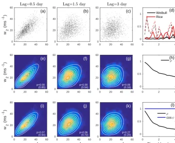
The temporal dependence structure of the wind speed at (39◦S, 216◦W) is illustrated in Fig. 6. As with the previous calculations, the pairs of lagged wind speeds

(w(tn), w(tn+s)) were subsampled to 2-day resolution to minimize the effect of serial dependence on the results of the goodness-of-fit tests. As the lag increases, the value of the dependence parameterρ decreases as expected for both the Weibull and Rice distributions (Fig. 6h, l). For most lags, the null hypothesis of the Weibull distribution as a model for the joint distribution is rejected (p <0.05; Fig. 6d). The rejection of the null hypothesis of a bivariate Weibull distri-bution is most robust for lags shorter than 3 days. In con-trast, the null hypothesis of a bivariate Rice distribution is rejected less often than it is not – although p <0.05 for more than one-third of the lags (Fig. 6d). Inspection of the example distributions shown demonstrates that the bivariate Weibull distributions are broader around their principal axis for small to intermediate wind speeds in a way that is not consistent with observations (Fig. 6e–g). Such structures are not seen in the best-fit Rice distributions (Fig. 6i–k). Note that for lags of 0.5 and 1.5 days the observed distributions suggest a flaring out of the joint distribution for large wind speeds that is accounted for by neither the bivariate Weibull nor Rice distributions. There is good evidence that these data were not drawn from a bivariate Weibull distribution, and the evidence that they are drawn from a bivariate Rice distribu-tion is not strong.p-values of fits obtained after shuffling of the lagged wind speed time series (in brackets in Fig. 6e– g, i–k and dashed lines in Fig. 6d) are generally larger than those of the unshuffled data: with a few exceptions (e.g. a lag of 1.75 days), the rejection of the null hypothesis of the full dataset being drawn from either of the parametric distri-butions considered is not associated with a failure to fit the marginals.

3.2 Wind speeds over land at 10 m and 200 m

Table 1.Maximum likelihood parameter estimates for the wind speed data shown in Figs. 5, 6, 7, and 8.

Sample Bivariate Rice Bivariate Weibull

Size (U1, σ1,U2, σ2, φ1−φ2+ψ, ρ) (a1, b1, a2, b2, ρ)

(m s−1, m s−1, m s−1, m s−1, –, –) (m s−1, –, m s−1, –, –) 500 hPa (39, 54.75◦S) 1625 (19.8, 10.5, 17.9, 11.3, 3.14, 0.71) (25.6, 2.5, 24.5, 2.3, 0.0)

(12, 15.75◦N) 1625 (0.0, 4.8, 6.9, 6.2, 0.88, 0.79) (6.8, 1.9, 11.0, 2.0, 0.62) (3◦S, 0.75◦N) 1625 (3.8, 3.1, 5.5, 3.5, 0.0, 0.75) (5.8, 2.1, 7.6, 2.3, 0.85) (15, 45◦S) 1625 (1.1, 4.2, 26.9, 11.0, 0.0, 0.15) (6.0, 1.8, 32.7, 3.1, 0.23)

500 hPa 0.5-day lag 1625 (19.4, 10.8, 19.4, 10.5, 0, 0.80) (25.1, 2.2, 24.9, 2.3, 0.90) 1.5-day lag 1624 (19.4, 10.9, 19.7, 10.4, 0, 0.40) (25.5, 2.4, 25.4, 2.5, 0.62) 3-day lag 1623 (19,3, 10.9, 19.4, 10.4, 0, 0.23) (25.6, 2.5, 25.3, 2.6, 0.44)

Cabauw night 1189 (1.9, 1.9, 6.9, 3.7, 0.0, 0.85) (3.1, 1.7, 8.9, 2.3, 0.92)

nightR1 763 (1.6, 1.2, 5.0, 4.0, 0.0, 0.83) (2.3, 2.2, 7.6, 2.1, 0.90)

nightR2 427 (3.5, 2.0, 9.4, 3.0, 0.0, 0.90) (4.6, 2.2, 10.9, 3.6, 0.95)

day 1060 (3.2, 2.8, 3.6, 4.7, 0.12, 0.98) (5.0, 2.3, 7.3, 2.1, 0.99) QuikSCAT (6.5◦S, 162◦W) 321 (7.2,1.5,6.7,1.7,1.27,0.48) (8.0,5.4,7.6,4.8,0.35)

(6.5◦S, 152◦W) 185 (7.3, 1.5, 7.0,1.7,1.15,0.95) (8.0,5.6,7.8,4.9,0.66) (6.5◦S, 142◦W) 208 (7.1,1.6,7.2,1.6,0.60,0.80) (7.9,5.1,8.0,5.0,0.83)

0 20 40

0 10 20 30 40 50

w 2

(ms

-1 )

(39 S, 54.75 S)◦ ◦

(a)

(e)

p=0.00 (0.35)

0 20 40

0 10 20 30 40 50

w 2

(ms

-1 )

(i)

p=0.30 (0.25)

0 20 40

w₁ (ms-1) 0

10 20 30 40 50

w 2

(ms

-1 )

0 10 20

0 10 20

30 (12 N, 15.75 N)

◦ ◦

(b)

(f)

p=0.01 (0.24)

0 10 20

0 10 20 30

(j)

p=0.02 (0.17)

0 10 20

w₁ (ms-1) 0

10 20 30

0 5 10 15

0 5 10 15

20 (3 S, 0.75 N)

◦ ◦

(c)

(g)

p=0.55 (0.10)

0 5 10 15

0 5 10 15 20

(k)

p=0.82 (0.16)

0 5 10 15

w₁ (ms-1) 0

5 10 15 20

0 10 20

0 20 40

60 (15 S, 45 S)

◦ ◦

(d)

(h)

p=0.13 (0.28)

Weibull

0 10 20

0 20 40 60

(l)

p=0.12 (0.27)

Rice

0 10 20

w₁ (ms-1) 0

20 40 60

Figure 5.Joint distributions of 500 hPa DJF 00Z wind speeds at four different pairs of latitudes along 216◦W. Wind speeds at the two latitudes quoted in the column headings are respectively denotedw1 andw2. (a–d)Scatterplots of wind speed data.(e–h)Maximum likelihood

bivariate Weibull pdfs (white contours) and kernel density estimates of the observed joint pdf (colours). Thep-value of a goodness-of-fit test with the null hypothesis that the observed wind speed data are drawn from the corresponding best-fit bivariate Weibull distribution is given. The values in brackets are thep-values obtained when the dependence structure is eliminated by shuffling the values ofw2in time.(i–l)As

0 20 40 60 0

20 40 60

w 2

(ms

-1 )

Lag=0.5day

(a)

(e)

p=0.00 (0.85)

0 20 40 60

0 20 40 60

w 2

(ms

-1

)

(i)

p=0.07 (0.94)

0 20 40 60

w

1 (ms

-1₎

0 20 40 60

w 2

(ms

-1 )

0 20 40 60

0 20 40 60

Lag=1.5day

(b)

(f)

p=0.00 (0.54)

0 20 40 60

0 20 40 60

(j)

p=0.06 (0.72)

0 20 40 60

w

1 (ms

-1₎

0 20 40 60

0 20 40 60

0 20 40 60

Lag=3day

(c)

(g)

p=0.09 (0.16)

0 20 40 60

0 20 40 60

(k)

p=0.27 (0.20)

0 20 40 60

w

1 (ms

-1₎

0 20 40 60

0 2 4

0 0.5 1

(d)

p Weibull Rice

0 2 4

0 0.5 1

(h)

Weibull

ρ

0 2 4

Time (days)

0 0.5 1

(l)

Rice

ρ cosψ

Figure 6.The temporal dependence structure of 500 hPa DJF 00Z wind speeds at (39◦S, 216◦W) for lagss=0.25 to 4 days, withw1=w(tn)

and w2=w(tn+s).(a–c) Scatterplots of wind speeds separated by 0.5 days (first column), 1.5 days (second column), and 3 days (third

column).(e–g)Maximum likelihood bivariate Weibull distribution (white contours) and kernel density estimate of the joint pdf of the lagged data. Thep-value of a goodness-of-fit test of the bivariate Weibull fit is quoted in white. The values in brackets are thep-values obtained when the dependence structure is eliminated by shuffling the values ofw2in time.(i–k)As in panels(e–g)for the bivariate Rice distribution.

Panels(d, h, l)show results at a range of different time lags.(d)p-values of bivariate goodness-of-fit tests for bivariate Weibull (solid black) and bivariate Rice (solid red). The dashed lines correspond to thep-values for shuffledw2. The thin black curve is the 0.95 significance level.

(h)Best-fit estimate of the parameterρof the bivariate Weibull distribution.(l)Best-fit estimates ofρ(black) and cosφ(blue) for the Rice distribution. Values of the best-fit model parameters are given in Table 1.

July, August, and September (JAS), separated into daytime (08:00–16:00 UTC) and nighttime (20:00–05:00 UTC) peri-ods. These data were subsampled in time to account for serial dependence. Only every 50th point was used in the follow-ing analysis. A small number of zero wind speed values were removed from the dataset.

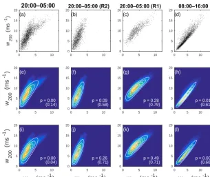
Monahan et al. (2011, 2015) demonstrated the existence of two distinct regimes of the nocturnal boundary layer in these data, corresponding to the very and weakly stratified boundary layers (vSBL and wSBL; e.g. Mahrt, 2014). These regimes, denoted respectively R1 and R2, were separated in Monahan et al. (2015) using a two-state HMM. Condi-tioning the data on the HMM state, the scatterplot of wind speeds at 10 and 200 m separates into two distinct popula-tions (Fig. 7a–c). The scatter of wind speeds at these two altitudes shows no evident regime structure during the day (Fig. 7d). In all cases, the wind speeds at the two altitudes are highly correlated.

p-0 5 10 0

5 10 15 20

w200

(ms

-1 )

20:00–05:00

(a)

0 5 10

0 5 10 15 20

20:00–05:00 (R2)

(b)

0 5 10

0 5 10 15 20

20:00–05:00 (R1)

(c)

0 5 10 15

0 5 10 15 20

08:00–16:00

(d)

p = 0.00 (0.14) (e)

0 5 10

0 5 10 15 20

w 200

(ms

-1 )

p = 0.09 (0.58) (f)

0 5 10

0 5 10 15 20

p = 0.28 (0.79) (g)

0 5 10

0 5 10 15 20

Weibull

p = 0.01 (0.61) (h)

0 5 10 15

0 5 10 15 20

p = 0.00 (0.04) (i)

0 5 10

w₁₀ (ms-1)

0 5 10 15 20

w 200

(ms

-1 )

p = 0.26 (0.71) (j)

0 5 10

w₁₀ (ms-1)

0 5 10 15 20

p = 0.49 (0.71) (k)

0 5 10

w₁₀ (ms-1)

0 5 10 15 20

Rice

p = 0.00 (0.60) (l)

0 5 10 15

w₁₀ (ms-1)

0 5 10 15 20

Figure 7.Joint distribution of JAS wind speeds at 10 and 200 m measured at Cabauw, NL.(a–d)Wind speed scatterplots.(e–h)Kernel

density estimate of the joint pdf of wind speeds (colour) and maximum likelihood bivariate Weibull distribution (contours). Thep-value of a goodness-of-fit test of the bivariate Weibull distribution is quoted in white. The values in brackets are thep-values obtained when the dependence structure is eliminated by shuffling the values ofw200in time.(i–l)As in the middle row, but for the best-fit bivariate Rice

distribution (contours).(a, e, i)All nighttime data (20:00–05:00 UTC).(b, f, j)Nighttime data conditioned on being in regimeR₂(very stable boundary layer).(c, g, k)Nighttime data conditioned on being in regimeR1(weakly stable boundary layer).(d, h, l)All daytime data

(08:00–16:00 UTC). Values of the best-fit model parameters are given in Table 1.

values of fits with w200 shuffled in time are all larger than those of fits to the original data; only for the Rice fit to the full nighttime data is the shuffled p-value below 0.05. As seen in the previous data considered, there is no systematic evidence that the failure of the joint Weibull or Rice distri-butions to model the joint distridistri-butions of the Cabauw data results from a failure to model the marginals.

3.3 Sea surface wind speeds

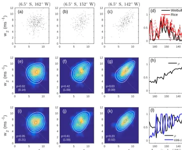
Twice-daily December, January, and February level 3.0 gridded SeaWinds scatterometer equivalent neutral 10 m wind speeds between 60◦S and 60◦N at a resolution of 0.25◦×0.25◦ from the National Aeronautics and Space Administration (NASA) Quick Scatterometer (QuickSCAT; Perry, 2001) are available from December 1999 through February 2008. Data flagged as having possibly been cor-rupted by rain were excluded from the following analysis. Although the data are nominally twice-daily, it is often the case that data for either the ascending or descending pass of the satellite are missing. The maximum likelihood parameter estimates of bivariate wind speed distributions and goodness-of-fit tests were carried out using every third non-missing data point in order to minimize the effect of serial

depen-dence. For the goodness-of-fit testsM=10 quantiles were used because of the relatively small sample sizes. Because of the near-polar orbit of the satellite results, observations of wind speed at different locations are not simultaneous. The joint distributions we consider therefore combine depen-dence in both space and time.

0 5 10 0

2 4 6 8 10 12

w 2

(ms

-1 )

(6.5 S, 162 W)◦ ◦

(a)

(e)

p=0.02 (0.14)

0 5 10

0 2 4 6 8 10 12

w 2

(ms

-1 )

(i)

p=0.05 (0.21)

0 5 10

w₁ (ms-1) 0

2 4 6 8 10 12

w 2

(ms

-1 )

0 5 10

0 2 4 6 8 10

12 (6.5 S, 152 W)

◦ ◦

(b)

(f)

p=0.42 (1.00)

0 5 10

0 2 4 6 8 10 12

(j)

p=0.61 (1.00)

0 5 10

w₁ (ms-1) 0

2 4 6 8 10 12

0 5 10

0 2 4 6 8 10

12 (6.5 S, 142 W)

◦ ◦

(c)

(g)

p=0.03 (0.00)

0 5 10

0 2 4 6 8 10 12

(k)

p=0.23 (0.02)

0 5 10

w₁ (ms-1) 0

2 4 6 8 10 12

140 150 160 0 0.5 1

(d)

p Weibull Rice

140 150 160 0 0.5 1

(h)

Weibull

ρ

140 150 160

Longitude (◦_W) 0

0.5 1

(l)

Rice

ρ

cosψ

Figure 8.Joint distribution of DJF QuikSCAT wind speeds at (6.5◦S, 135◦W), denotedw1, and westward along a zonal transect to 165◦W

(denotedw2).(a–c)Scatterplots of wind speed at (6.5◦S, 135◦W) and at the points (6.5◦S, 162◦W), (6.5◦S, 152◦W), and (6.5◦S, 142◦W).

(e–g)Kernel density estimate of the joint pdf (colour) as well as the maximum likelihood bivariate Weibull distribution (white contours). The

p-value of a goodness-of-fit test of the bivariate Weibull distribution is quoted in white. The values in brackets are thep-values obtained when the dependence structure is eliminated by shuffling the values ofw2in time.(i–k)As in panels(e–g) but for the bivariate Rice distribution.

(d)p-values of the bivariate goodness-of-fit tests for the wind speeds along the transect, for the bivariate Weibull distribution (solid black) and for the bivariate Rice distribution (solid red). The dashed lines correspond to thep-values for shuffledw2.(h)Estimate of the parameter

ρfrom the best-fit bivariate Weibull distribution along the transect.(l)Estimate of the parametersρ(black) and cosψ(blue) from the best-fit bivariate Rice distribution along the transect. Values of the best-fit model parameters are given in Table 1.

speeds than for larger values, a feature not evident in the best-fit bivariate Rice distributions (Fig. 8i–k) or the scatter of data (Fig. 8a–c). From these results, we find only equivocal evidence that the pairs of wind speed data along this zonal transect are drawn from a bivariate Weibull distribution and no strong evidence to reject the null hypothesis that they are drawn from a bivariate Rice distribution. Again, thep-values of fits to temporally shuffled wind speeds are generally sim-ilar to or larger than those of fits to the full distribution. The bivariate Rice distribution with the wind speed at 142◦W (Fig. 8k) illustrates a rare example in which the parametric fit to the original data passed the goodness-of-fit test at the 5 % significance level while the fit to the shuffled data did not; it is evident from Fig. 8d that this situation is not com-mon. The surface wind vector components in the tropics are known to be non-Gaussian (e.g. Monahan, 2007), so we have a priori reasons to believe the joint distribution should not be Ricean. The fact that the data do not generally allow for a

rejection of the null hypothesis that the winds are bivariate Rice (for either the original or shuffled datasets) is likely a consequence of the relatively small sample size.

0.4 0.6 0.8 1

ρ

0.4 0.6 0.8 1

cos

ψ

N = 250

(a)

0.4 0.5 0.6

C orr(w1, w2) (sample)

0.4 0.5 0.6

Co

r

r

(

w1

,w

2

)

(a

pp

ro

x)

(g) (d)

4 6 8 10

w1

4 6 8 10

w2

0.4 0.6 0.8 1

ρ

0.4 0.6 0.8 1

N = 1500

(b)

0.4 0.5 0.6

C orr(w1, w2) (sample)

0.4 0.5

0.6 (h)

(e)

4 6 8 10

w1

4 6 8 10

0.4 0.6 0.8 1

ρ

0.4 0.6 0.8 1

N = 9000

(c)

0.4 0.5 0.6

C orr(w1, w2) (sample)

0.4 0.5

0.6 (i)

(f)

4 6 8 10

w1

4 6 8 10

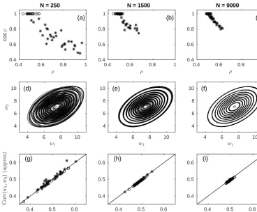
Figure 9. (a–c) Estimates of ρ and cosψ from 50 realizations of bivariate Ricean variables with(U1, σ1,U2, σ2, ρ, φ1−φ2+ψ )=

(7.3,1.5,6.9,1.5,0.4,0)for each of the sample sizesN=250,1250, and 9000. The open circles correspond to estimates with cos(φ1−

φ2+ψ )≥0.99, while the stars are estimates with cos(φ1−φ2+ψ ) <0.99.(d–f)Contours of bivariate Rice pdfs corresponding to 10 of the

50 best-fit parameter estimates (randomly chosen). The contour values are the same for all pdfs within each subplot.(g–i)Scatterplot of the sample correlation coefficient between the two Ricean variables and the correlation coefficient given by the approximate expression Eq. (40). The 1 : 1 line is given in solid black. The open circles and stars are as in the upper row.

smaller as the sample size increases(Fig. 9b, c). Despite the large variation ofρand cosψfor small to intermediate sam-ple sizes, there is relatively little variation in the structure of the corresponding bivariate Rice distributions (Fig. 9d–f).

An indication of why increases inρshould counterbalance decreases in cosψwith only small effects on the joint distri-bution is given by the approximate expression for the corre-lation coefficient, Eq. (40). The value of this approximation is unaffected by changes inρandψ that leave the numera-tor invariant. The compensation between sampling variations inρand cosψis evident the fact that corr(w1, w2)given by Eq. (40) is an excellent approximation to the sample corre-lation coefficient even for estimates of ρ and cosφ which are far away from the population values (Fig. 9g–i). Note that there is no evident relationship between sampling fluc-tuations in corr(w1, w2)and those ofρandψ: the range of sample correlation values for(ρ,cosψ )near the population values of (0.5,1) (open circles) is the same as that for values of(ρ,cosψ )far from these values (stars). In these parameter ranges, the dependence betweenw1andw2constrainsρand

ψnot individually, but together – over large ranges of values for sufficiently small sample sizes.

4 Conclusions

wind speeds (over land and over the ocean; at the surface and aloft; in space and in time) the bivariate Rice distribu-tion was shown to generally model the observadistribu-tions better than the bivariate Weibull distribution. However, in many cir-cumstances the differences between the two distributions are small and the convenience of the bivariate Weibull distribu-tion relative to the bivariate Rice distribudistribu-tion is a factor which may motivate its use.

The fact that the bivariate Rice distribution is easier to work with, but less flexible, than the bivariate Weibull dis-tribution is evident from inspection of their analytic forms and the relative number of parameters to fit (five vs. six). If the bivariate Weibull distribution was generically appropri-ate for modelling the bivariappropri-ate wind speed distribution, there would be no need to consider more complicated models such as the bivariate Rice. This study provides an empirical as-sessment of the relative practical utility of the two models, trading off the ability to model more general dependence structures (e.g. negatively correlated speeds) against model simplicity. Neither the univariate nor the bivariate Weibull or Rice distributions are expected to represent the true distribu-tions of wind speeds (e.g. Carta et al., 2009). The results of this analysis characterize the practical utility of these models, rather than making a claim to their “truth”. It is noteworthy that for the data considered in this study, the failure of either the bivariate Rice or Weibull distributions to adequately fit the joint distribution of wind speeds (at a significance level of 5 %) is not generally associated with a corresponding fail-ure of the parametric distribution to model the marginals. An interesting direction of future study would be consideration of other parametric models for the joint distribution of non-negative quantities, such as the α-µ distribution (Yacoub, 2007), copula-based models (e.g. Schlözel and Friederichs, 2008), or distributions obtained through nonlinear transfor-mations of multivariate Gaussians (e.g. Brown et al., 1984).

Many of the assumptions that have been made regarding the distribution of the wind components are known not to hold in various settings. For example, the vector wind com-ponents are generally not Gaussian, either aloft or at the sur-face (e.g. Monahan, 2007; Luxford and Woollings, 2012; Perron and Sura, 2013), and fluctuations will not generally be isotropic (especially over land; cf. Mao and Monahan, 2017). Furthermore, when used to model temporal depen-dence the assumed correlation structure cannot account for the anisotropy in autocorrelation of orthogonal components in either space (e.g. Buell, 1960) or time (e.g. Monahan, 2012b). Relaxing the assumptions regarding isotropy of cor-relation structure results in expressions for the joint speed distributions involving integrals over angle which are not an-alytically tractable.

While it is possible to relax the assumption of Gaussian components for univariate speed distribution (e.g. Monahan, 2007; Drobinski et al., 2015), extending this analysis to the bivariate case would involve specifying a non-Gaussian de-pendence structure for the components. At present, there is no physically based model for such dependence. Without any such physical justification, the only option is an empirical in-vestigation of the ability of different copula models to repre-sent observed joint wind speed distributions. It is unlikely that a copula-based model for dependence of components will admit analytically tractable expressions for joint speed distributions. A copula-based analysis of either the compo-nents or the speeds directly is also likely necessary for mod-elling extreme wind speeds (either large percentiles, peaks over threshold, or block maxima), as the tails of the bivariate Rice and Weibull distributions may not be adequate for this task. Finally, extending the approach used in this study to ob-tain explicit closed-form results for the bivariate wind speed distribution to a higher-dimensional multivariate setting – of wind speeds alone, or of a mixture of wind speeds and other meteorological quantities – will be analytically intractable for any except the simplest (and likely unrealistic) covari-ance structures. It may not be practical to extend the program of obtaining closed-form expressions for joint speed distri-butions from models of the component distridistri-butions much further beyond the bivariate Rice and Weibull speed distribu-tions considered in this study.

Ultimately, it would be best for models of the joint distri-bution of wind speeds to arise from physically based (if still idealized) models, as has been done for the univariate case in Monahan (2006) and Monahan et al. (2011). The devel-opment of such models represents an interesting direction of future study.

Data availability. The ERA-Interim 500 hPa zonal and

Appendix A: Numerical computation of bivariate Rice pdf

Equation (25) is difficult to evaluate numerically when the arguments of the Bessel functions become large. We have found that a computationally more stable result is obtained when this equation is expressed in the form

p(w1, w2)=

w1w2

2π σ₁2σ₂2(1−ρ2₎ 2π Z

0

expf (w1, w2, λ)dλ, (A1)

where

f (w1, w2, φ)= − 1 2(1−ρ2₎

"

w₁2+U2₁

σ₁2 +w

2 2+U

2 2 σ₂2

−2ρU1U2cos(φ1−φ2+ψ ) σ1σ2

#

+lnI0pA2_+B2_+2ABcosλ

+Ccosνcosλ+ln cosh(Csinνsinλ)dλ, (A2) with

A= w1

q

a2₁+b2₁ σ1

, (A3)

B= w2

q

a₂2+b₂2

σ2 , (A4)

C= ρ 1−ρ2

w1w2

σ1σ2 , (A5)

and the integral is evaluated numerically. Equation (A1) is obtained from Eq. (26) using the fact that

Ik(x)Ik(y)=

1 2π

2π Z

0

I₀(

q

x2_+y2_{+2xycosφ)coskφdφ (A6)}

(which follows from Eq. 33) and use of Eq. (24). Whenwi/σi becomes large, numerical evaluations of the Bessel function in Eq. (A1) become unreliable. For the present computations using Matlab, values of Inf occur in such cases. This problem was not solved by using the approximation Eq. (10) when the argument of the Bessel function is large, as this approxima-tion is not sufficiently accurate.

Appendix B: Bivariate goodness-of-fit test

Goodness-of-fit of the bivariate distributions considered was assessed as follows. For the speed dataset wj,n, j =1,2 andn=1, . . ., N, evenly spaced quantiles qj,i=i/M, i= 0, . . ., M for the marginals are estimated. The quantiles qj,0=0 andqj,M=1 are estimated respectively as 0.9 times the smallest observed value and 1.1 times the largest ob-served value. The number of pairs of observations falling si-multaneously into all pairs of quantiles are computed:

fkl= (B1)

N

X

n=1 1

w1,n∈(q1,k, q1,(k+1)]∩ w2,n∈(q2,l, q2,(l+1)],

where1(·)is the indicator function. The pdf with maximum likelihood parametersθ is then integrated to obtain the ex-pected number of observations in these intervals

gkl=N q1,(k+1)

Z

q1,k

q2,(l+1)

Z

q2,l

p(w1, w2;θ )dw1dw2 (B2)

and the test statisticAis computed:

A= 1 M2

M

X

k,l=1

|fkl−gkl|. (B3)

Any elementsgklwhich take the value of Inf (because of nu-merical difficulties in evaluating the Bessel function for large arguments; cf. Appendix A) are excluded from the calcula-tion of the test statisticA.

After computation ofAfrom the observations, an ensem-ble ofB random realizations of lengthN fromp(w1, w2;θ ) is generated and the correspondingAek,k=1, . . ., Bvalues of the test statistic are generated in the manner described above. Thep-value of the null hypothesis that the observations are drawn from the specified distribution is finally computed as the fraction of Aek values falling above A. Throughout this analysis, we useM=20 andB=250 (unless otherwise noted). This goodness-of-fit test assumes independence of the random draws(w1n, w2n), (w1m, w2m),m6=n. To min-imize the effect of serial dependence in data, in this study we subsample the datasets considered with a sampling interval sufficiently large to balance reducing serial dependence with maintaining sample size.