https://doi.org/10.5194/npg-25-521-2018 © Author(s) 2018. This work is distributed under the Creative Commons Attribution 4.0 License.
Laboratory and numerical experiments on stem waves due to
monochromatic waves along a vertical wall
Sung Bum Yoon1, Jong-In Lee2, Young-Take Kim3, and Choong Hun Shin1
1Department of Civil and Environmental Engineering, Hanyang University, EIRCA Campus, Ansan, Gyeonggi, 15588, South Korea
2Department of Marine and Civil Engineering, Chonnam National University, Yeosu Campus, Yeosu, Jeonnam, 59626, South Korea
3River and Coastal Research Division, Korea Institute of Civil Engineering & Building Technology, Goyang, Gyeonggi, 10223, South Korea
Correspondence:Choong Hun Shin ([email protected]) Received: 6 July 2017 – Discussion started: 1 August 2017
Revised: 25 May 2018 – Accepted: 11 June 2018 – Published: 27 July 2018
Abstract. In this study, both laboratory and numerical ex-periments are conducted to investigate stem waves propa-gating along a vertical wall developed by the incidence of monochromatic waves. The results show the following fea-tures: for small-amplitude waves, the wave heights along the wall show a slowly varying undulation. Normalized wave heights perpendicular to the wall show a standing wave pat-tern. The overall wave pattern in the case of small-amplitude waves shows a typical diffraction pattern around a semi-infinite thin breakwater. As the amplitude of incident waves increases, both the undulation intensity and the asymptotic normalized wave height decrease along the wall. For larger-amplitude waves with smaller angle of incidence, the mea-sured data clearly show stem waves. Numerical simulation results are in good agreement with the results of laboratory experiments. The results of present experiments favorably support the existence and the properties of stem waves found by other researchers using numerical simulations. The char-acteristics of the stem waves generated by the incidence of monochromatic Stokes waves are compared with those of the Mach stem of solitary waves.
1 Introduction
Coastal structures have been increasingly constructed in deep water regions as the size of ships becomes larger. In such deep water regions, a vertical-type structure is preferred to
save construction costs. In the case of a vertical structure, stem waves occur when waves propagate obliquely against the structure. Thus, there is a need for careful considera-tion to secure appropriate free board and stability of caisson blocks.
in-troduced a parabolic approximation equation based on the Boussinesq equation and analyzed stem waves for the case of cnoidal incident waves. Yoon and Liu (1989) showed the importance of the incident wave nonlinearity. Most previ-ous studies on stem waves focused on the properties of stem waves depending on the incident angle and wave nonlinearity of monochromatic waves.
While the stem waves generated by the sinusoidal waves have drawn less attention in recent years, the Mach stem induced by the interaction between the line solitons in the shallow-waters has continuously attracted the attention of the researchers. Since the pioneering work of Miles (1977a, b) on the obliquely interacting solitary waves, the soliton in-teractions have been extensively studied. Miles (1977b) de-veloped an analytical solution to predict the amplification of the stem wave along the wall as a function of the interaction parameter, k∗=θ0/
√
3H0/ h, where H0, h, and θ0 are the wave height, the water depth, and the incident angle of soli-tary wave, respectively. Whenk∗=1, the amplification of a solitary wave can reach 4 times that of the incident wave. Soomere (2004) investigated the soliton interactions based on the KP equation (Kadomtsev and Petviashvili, 1970). Ko-dama et al. (2009) and KoKo-dama (2010) proposed the mod-ified interaction parameter,κ∗=tanθ0/(
√
3H0/ hcosθ0). Li et al. (2011) conducted a precision laboratory experiment to capture the detailed features of Mach reflection using the LIF (laser-induced fluorescent) technique. The laboratory data of Li et al. (2011) strongly support the theory of Miles (1977b) except the cases where the κ∗ value lies in the neighbor-hood of the 4-fold amplification. Funakoshi (1980), Tanaka (1993), Li et al. (2011), and Gidel et al. (2017) performed nu-merical experiments to verify the Miles’ 4-fold amplification. As summarized by Li et al. (2011) and Gidel et al. (2017) most of the models underestimated the 4-fold amplification due to the limitations of the computational resources. The amplification ratio of 3.6 obtained by Gidel et al. (2017) is so far the maximum among the numerical results showing the full development stage of stem waves.
Even though the existence and the properties of stem waves for sinusoidal waves are well known theoretically via numerical simulations (e.g., Yue and Mei, 1980; Yoon and Liu, 1989), they are not yet fully supported by physical ex-periments. Berger and Kohlhase (1976) conducted hydraulic experiments to show the existence of stem waves for the cases of sinusoidal waves. Their experimental data, however, failed to produce clear stem waves, possibly due to partial re-flection from the beach, diffraction from the ends of vertical wall, or insufficient space in the wave basin. Lee et al. (2003), Lee and Yoon (2006) and Lee and Kim (2007) performed lab-oratory experiments to investigate stem waves for sinusoidal waves and compared the measured waves with the numerical results obtained using a nonlinear parabolic approximation equation model. Their hydraulic experiments demonstrated stem waves for some cases with a relatively large incident wave. However, the stem waves were not clearly developed
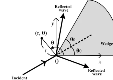
Figure 1.Definition sketch of wave field around a vertical wedge.
because of both the narrowness of the wave basin and the reflected waves from the beach. Only four cases of incident wave conditions were tested in their experiment. Thus, the experimental data were not sufficient to investigate the prop-erties of stem waves. Moreover, the numerical results for the cases of large angle of incidence were not highly accurate be-cause of the small-angle parabolic model employed for their numerical simulations. Thus, there is still need to perform a precisely controlled experiment to investigate the existence and the properties of stem waves.
In this study, precisely controlled laboratory experiments are conducted to investigate the characteristics of stem waves developed by the incidence of monochromatic waves. The measured data are compared with numerical simulations and analytical solutions. In the following section, the numerical simulation method and the analytical solution employed in this study are summarized. In Sect. 3, the experimental setup and procedure are briefly presented. In Sect. 4, the measured wave heights are compared with numerically simulated re-sults and analytical solutions. In Sect. 5, the characteristics of the stem waves generated by the incidence of monochro-matic Stokes waves are compared with those of the Mach stem of solitary waves. In the final section, the major find-ings from this study are summarized.
2 Numerical simulation and analytical solution
In this study, the stem waves that have developed along a vertical wall over a constant water depth are investigated for the cases of monochromatic waves. Figure 1 shows a sketch of the wave field around a vertical wedge. The monochro-matic waves are symmetrically incident towards the tip of the wedge. Thexaxis of the coordinate system is aligned with a side wall of the wedge. The angle of incidenceθ0is defined as the angle between thex axis and the incident wave ray. The computational domain lies in the region of 0≤ x and
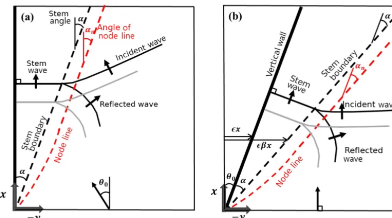
Figure 2.Coordinate system for numerical simulations:(a)present,(b)Yue and Mei (1980).
2.1 Numerical simulation method
To compare with our experiments, the latest version of REF/DIF, a wide-angle nonlinear parabolic approximation equation model developed by Kirby et al. (2002), is em-ployed to simulate stem waves. The REF/DIF model can deal with the refraction–diffraction of Stokes waves of third-order nonlinearity over a slowly varying depth and current. Due to the use of parabolic formulation the reflection in the main di-rection of propagation is forbidden, but not in the transverse direction. In this study, the water depth is uniform, and no ambient current is present. With no current and energy dis-sipation on a constant water depth and by selecting a (1, 1) Padé approximant in the model, the governing equation of the REF/DIF model is simplified as
2ik∂A ∂x +
∂2A ∂y2 +
i
2k ∂3A ∂x∂y2−
ωk3 Cg
D|A|2A=0, (1)
wherehis the water depth,i= √
−1,Cgis the wave group velocity,Ais the complex wave amplitude, andkandωare the wave number and the angular frequency, respectively, and satisfy the following linear dispersion relationship:
ω2=gktanhkh, (2)
wheregis the gravitational acceleration, andDis given as
D=cosh 4kh+8−2tanh 2kh
8sinh4kh . (3)
The third term of Eq. (1) is the correction term ob-tained by selecting the (1, 1) Padé approximant for the wide-angle parabolic approximation. According to Fig. 2 of Kirby (1986) the accuracy of the waves propagating
obliquely to the main direction of propagation, i.e.,x direc-tion, can be maintained up to±45◦. In this study the range of the incidence angles of both incident and reflected waves lies from±10 to±40◦. Thus, the sufficient accuracy of the numerical solution is expected.
The conventional parabolic approximation equation, i.e., the nonlinear Schrödinger equation of Yue and Mei (1980), is obtained if this term is neglected. The last term in Eq. (1) describes the nonlinear self-interaction of waves. Figure 2 shows the coordinate system for the present numerical sim-ulation in comparison with that of Yue and Mei (1980). In the present simulation the incident waves are prescribed obliquely along theyaxis as
A=a0eiknysinθ0, (4)
wherea0is the amplitude of the incident wave, andknis the
wave number with the nonlinear correction given as
kn=k
1− C 2Cg
D(k|A|)2
, (5)
whereC(=ω/ k)is the phase speed of wave. The no-flux boundary condition is prescribed along the vertical wall (y= 0) given as
∂A
∂y =0. (6)
If the side boundary opposite to the vertical wall is located far from the wall, the no-flux boundary condition, Eq. (6), can also be used. However, to save the computational re-sources the obliquely incident plane wave condition is pre-scribed along the side boundary aty= −ymaxas
Along the outer side no boundary condition is necessary, because Eq. (1) is a parabolic-type differential equation. The grid size,1x and1y, isL/80 whereL is the wave length of an incident wave. The size of the computational domain is 50Lin thexdirection, and 400Lin theydirection.
For the latter we use the nonlinear parameter,K, proposed by Yue and Mei (1980) and given as
K=
ka0 tanθ0
2 CD
Cg
. (8)
K is the single parameter representing both the nonlinearity of incident wave and the angle of incidence on the formation of stem waves along the vertical wall. This nonlinear parame-ter was obtained by Yue and Mei (1980) from the dimension-less form of the small angle version of Eq. (1). The details of the derivation ofKcan be found in Yue and Mei (1980). 2.2 Analytical solution
Chen (1987) developed an analytical solution for the Helmholtz equation in polar coordinates to solve the com-bined reflection and diffraction of monochromatic waves due to a vertical wedge. The analytical solution is given in a polar coordinate as shown in Fig. 1 as
8 r, θ∗, z, t= −iga0
ω
cosh{k (z+h)} coshkh F r, θ
∗
eiωt, (9) where8 (r, θ∗, z, t )is the velocity potential, andF (r, θ∗)is a diffraction factor (i.e.,A/a0) given as
F r, θ∗ (10)
=2
ν "
J0(kr)+2 ∞ X
n=1
einπ/2νJn/ν(kr)cos nα∗ ν cos nθ∗ ν # ,
whereθ∗=θ−2θ0,α∗=π−θ0,ν=2(π−θ0)/π, andθ0 is the angle of incidence. J0(kr)is the Bessel function of the first kind of order 0. The absolute value of the diffrac-tion factor |F (r, θ∗)| represents the normalized wave am-plitude|A|/a0, or the normalized wave heightH /H0where
H0(=2a0) is the wave height of the incident wave. The ana-lytical solution of Chen (1987) is linear. Thus, this anaana-lytical solution does not allow the formation of stem waves. The de-tails of the derivation of the analytical solution can be found in Chen (1987).
3 Hydraulic experiments
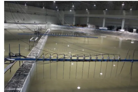
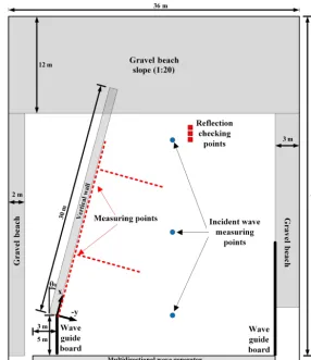
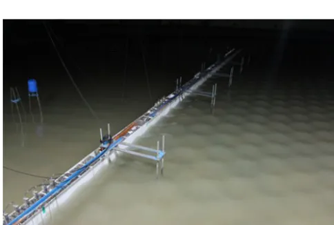
Hydraulic experiments are carried out in the multidirectional irregular wave generation basin of the Korea Institute of Con-struction Technology (see Fig. 3). The basin used in the labo-ratory experiments is 42 m long, 36 m wide, and 1.05 m high. A snake-type wave generator consisting of 60 wave boards, each with dimensions of 0.5 m in width and 1.1 m in height
Figure 3.Experimental facility and wave gauge array.
and driven by an electronic servo piston, is installed along the 36 m long bottom wall of the wave basin. Free surface dis-placements are measured using 0.6 m long capacitance-type wave gauges with a measuring range of±0.3 m.
Figure 4 shows the configuration of the experimental setup and model installation. A 30 m long vertical wall is installed along the left lateral side of the basin in four different orien-tations. A dissipating gravel beach with a 1/20 slope is ar-ranged on the opposite side of the wave generator to reduce the reflection of waves inside the basin. Another dissipating beach and wave absorber are also set along the lateral sides and at the back of the wave generator. Along the lateral side opposite to the vertical wall a 10 m long wave guide is in-stalled to avoid diffraction from the side wall. Note thatθ0is the angle between the vertical wall and the incident waves. The origin of the spatial coordinate system of the labora-tory experiments (i.e.,x0,y0) is set at the tip of the verti-cal wall which is located 3 m and 5 m away from the lateral side and the wave generator, respectively, as shown in Fig. 4. The width and height of the vertical wall were both 0.6 m. The experiments are carried out at a constant water depth of
h=0.25 m. The free board from a still water level to the top of the vertical wall is 0.35 m in order to prevent overtopping of waves.
The incident wave conditions are summarized in Table 1. The title of each test case is composed of three alphabet characters and a numeric digit. The first letter, M, stands for “monochromatic” waves. The letters S or L represents “shorter” or “longer” waves in terms of period, respectively. The letters S, M, or L represents “small”, “medium”, or “large” waves in terms of wave height, respectively. Finally, the numeric digit represents the angle of incidence.
Table 1.Experimental wave conditions (h=0.25 m).
Nonlinearity
Test Wave period Wave height Incident angle Wave steepness Nonlinear
case T (s) H0(m) θ0(deg.) kH0 parameterK
MSS1 0.7 0.009 10 0.076 0.088
MSS2 20 0.021
MSS3 30 0.008
MSS4 40 0.004
MSM1 0.027 10 0.229 0.793
MSM2 20 0.186
MSM3 30 0.074
MSM4 40 0.035
MSL1 0.036 10 0.305 1.411
MSL2 20 0.331
MSL3 30 0.132
MSL4 40 0.062
MLS1 1.1 0.018 10 0.076 0.123
MLS2 20 0.029
MLS3 30 0.011
MLS4 40 0.005
MLM1 0.054 10 0.228 1.108
MLM2 20 0.260
MLM3 30 0.103
MLM4 40 0.049
MLL1 0.072 10 0.304 1.969
MLL2 20 0.462
MLL3 30 0.184
MLL4 40 0.087
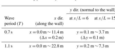
Table 2.Measuring points in hydraulic experiments.
ydir. (normal to the wall)
Wave xdir. atx/L=6 atx/L=15
period (T) (along the wall)
0.7 s x=0.0 m∼11.4 m y=0.1 m∼3.7 m (1x=0.2 m) (1y=0.1 m) 1.1 s x=0.0 m∼22.8 m y=0.2 m∼7.3 m
(1x=0.4 m) (1y=0.2 m)
is 40L for the case of T =0.7 s and 20L for the case of
T =1.1 s, whereLrepresents the wavelength of monochro-matic waves corresponding to the given periodT. The inci-dent angles ofθ0=10, 20, 30, and 40◦are obtained by ad-justing the orientation of the vertical wall. Thus, the incident waves propagate normal to the line of the wave generator. The nonlinearity of the incident waves are presented in two dimensionless parameters, wave steepnesskH0and the non-linear parameterKgiven by Eq. (8).
In the real world, we can assume the situation where the swell is incident on a breakwater. Swell waves are the regu-lar longer period waves created by storms far away from the
beach. Swell waves tend to have longer periods than wind waves. The wave period of swell lies between 10 to 15 s. Breakwaters are generally constructed at a depth of about 10 to 20 m. If the wave height is 1 to 3 m, the swell wave con-ditions can be within the range of Stokes wave, as shown in Fig. 5. In the figure the empty blue circles represent the swell wave conditions and the red triangles represent the incident waves tested in this study. It can be seen that the incident waves tested in this study belong to the Stokes range. The dispersion effect of the Stokes waves is much stronger than that of the solitary waves. Thus, the characteristics of stem waves in this study should be very different from those of the solitary waves. In Fig. 5, thexaxis represents the relative water depth (ratio of water depth to deep water wave length, i.e., the measure of wave dispersion). They axis represents the wave steepness (ratio of wave height to deep water wave length, i.e., the measure of wave nonlinearity).
Figure 4.Definition sketch of the experimental setup.
1.1 s, respectively, along the wall, and 1y=0.1 and 0.2 m for T =0.7 and 1.1 s, respectively, normal to the wall. Ta-ble 2 gives a summary of the wave height measurement posi-tions. The wave heights are extracted from the measured free surface displacements using the zero-upcrossing method. In this method a wave is defined when the surface elevation crosses the zero line or the mean water level upward and continues until the next crossing point. This method is a widely accepted method for extracting representative statis-tics from raw wave data. Figure 6 shows the hexagonal or beehive wave pattern captured during the experiment in front of a vertical wall for the case of θ0=30◦. This is typical of the cross sea generated by the oblique interaction of two or more traveling plane waves (see, e.g., Le Mehauté, 1976; Mei, 1983; Nicholls, 2001). Postacchini et al. (2014) studied the dynamics of crossing wave trains on a plane slope in shal-low waters. The stem waves can develop at the intersection of two crest lines of the crossing waves. When the crossing waves propagate towards a shore, they experience shoaling and break. Postacchini et al. (2014) proposed an analytical theory based on ray convergence to identify the position and the crest length of the breaker. The stem waves in the present study are developed by the oblique nonlinear interaction
be-tween the incident and the reflected waves. Thus, the gener-ation mechanism is similar to Postacchini et al. (2014).
Figure 5.The present experiment and wave conditions of the real-world cases (after Le Méhauté, 1976). The solid red triangles rep-resent the incident waves tested in this study and empty blue circles represent the swell wave conditions. Thexaxis represents the rel-ative water depth (ratio of water depth to deep water wave length, i.e., the measure of wave dispersion). Theyaxis represents the wave steepness (ratio of wave height to deep water wave length, i.e., the measure of wave nonlinearity).
Figure 6.Wave pattern in front of a vertical wall (θ0=30◦).
to the gravel beach is less than the maintained 3 % for all the waves considered in the experiments.
4 Results and discussions
In this study, experiments on the formation of stem waves near a vertical wall are conducted and the measured wave heights are compared with results calculated using both
Figure 7.Definition sketch for the stem angle and the stem bound-ary.
the wide-angle parabolic approximation equation numerical model, REF/DIF, and the analytical solution of Chen (1987). All the figures for the experimental and calculated data are presented in the Supplement to avoid an excess of figures.
Prior to presenting the experimental and numerical results, the definitions of the stem angle and the stem width are dis-cussed. The definition of stem width is rather controversial. Yue and Mei (1980) defined the stem width as the distance from the wall to the edge of the uniform wave amplitude re-gion. However, it is not an easy task to locate the edge of the flat region. Berger and Kohlhase (1976) defined the stem width for the periodic waves as the distance along the stem crest lines from the wall to the first node line of the standing wave pattern, which is easier to identify from the measured data. However, Soomere (2004) obtained the analytical stem length using the KP equation for the obliquely interacting two solitary waves. As pointed out by Li et al. (2011) the crest lines of the stem wave, the incident, and the reflected solitons measured in their experiment are not straight, and they do not meet at a point. In reality, the analytical solutions of the KP equation deviate slightly from the pattern observed in the experiment. Thus, Li et al. (2011) proposed the edge of the Mach stem as the intersection of the linear extensions of the stem and the incident-wave crest lines.
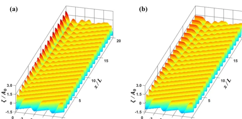
Figure 8.Three-dimensional plots of normalized wave height for(a)MLS1 and(b)MLL1 cases from simulation.
Figure 9.Three-dimensional plots of normalized free surface displacements(a)MLS1 and(b)MLL1 cases from simulation.
in Figs. 2a and 7, when the stem waves are fully developed, the stem boundary is nearly parallel to the first node line. Thus, as suggested by Berger and Kohlhase (1976), the ex-perimental stem angle α is determined in this study as the angle of node line,αn. The node line is roughly determined using the node points from the wave height data measured along two lines ofx=6 and 15L. When the distances be-tween the first node points and the wall are λ6andλ15 for two sections ofx=6 and 15L, respectively (see Figs. S5 and S6), then the angle of the node line,αn, can be determined as
α≈αn=tan−1 λ
15−λ6 9L
. (11)
Thisαndecreases as the waves propagate along the wall. It reaches an asymptotic value after the waves propagate
ap-proximately 30 wave lengths. Thus, the experimentalαn de-termined by Eq. (11) is slightly overestimated forx≤30L.
In this study the stem angle,α, is defined as the asymp-totic angle of node line as shown in Fig. 7. To estimate the asymptoticαnthe numerical calculation is conducted using the domain extended up to 50Lin thex direction, and the instantaneous free surface displacements are calculated and plotted as shown in Fig. 7. Using two distances between the node points and the wall, λ30 andλ50 for two sections of
x=30 and 50L, respectively, the stem angleαis determined as
α=αn=tan−1 λ
50−λ30 20L
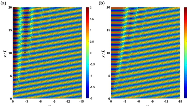
Figure 10.Contour plots of the instantaneous normalized free surface for(a)MLS1 and(b)MLL1 cases from simulation.
Figure 11.Comparison of calculated and measured normalized wave heights along the wall as a function of nonlinear parameterK. Black solid curve represents the wave height predicted by shock theory of Yue and Mei (1980), red and blue solid curves denote the calculated wave heights forθ0=10 and 20◦, respectively. Symbols are measured data.
The stem widthλscan be determined using the stem angle
αas
λs=xtanα. (13)
4.1 Shorter waves (T =0.7 s)
Figure S1 shows the comparisons between the measured, numerically simulated, and analytically calculated wave heights, H / H0, along the vertical wall for the cases of
H0=0.009 m with T=0.7 s (i.e., MSS series). The
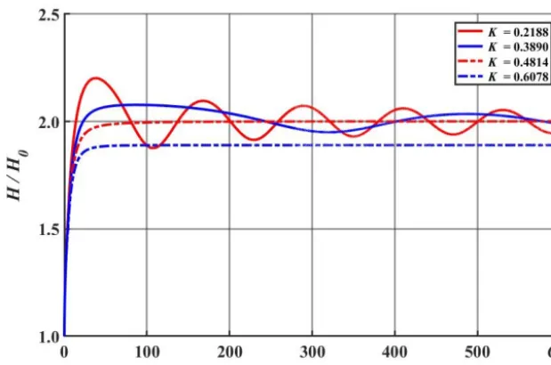
undu-Figure 12.Comparison of calculated normalized wave heights along the wall for various nonlinear parameter values ofK(θ0=10◦).
lation with the average value of H /H0=2.0. The maxi-mum value of undulation is approximatelyH /H0≈2.3, and the location of maximum wave height decreases with in-creasing angle of incidence. In particular, the overall pat-tern of wave height distribution does not support the gen-eration of stem waves, which are characterized by uniform wave heights smaller than those obtained from linear diffrac-tion theory (Yue and Mei, 1980; Yoon and Liu, 1989). The wave heights calculated using the REF/DIF numerical model (Kirby and Dalrymple, 2002) and the analytical solution of Chen (1987) agree well with the measured wave heights. This supports the idea that the effects of nonlinearity of inci-dent waves are too weak to develop stem waves. In the case of θ0 =10◦, the maximum normalized wave heights does not reachH /H0≈2.3 because the size of the experimental area is insufficient. If the vertical wall is sufficiently long, the same result could apparently be obtained forθ0 =10◦.
Figures S2 and S3 show the comparisons of wave heights
H /H0 along a line (x=6, 15L) perpendicular to the ver-tical wall. The distribution of wave height shows the typ-ical pattern of standing waves formed by superposition of the reflected waves on the incident waves. Berger and Kohlhase (1976) called these standing waves stem waves as long as they propagated parallel to the wall. If stem waves, however, are defined as waves with a uniform wave height in the direction normal to the wall, then the wave height distri-butions for these small-amplitude waves in MSS series show no sign of stem waves. The wave amplitude for this MSS se-ries is too small to generate stem waves along the wall.
Figure S4 shows normalized wave heights along the ver-tical wall for the cases of MSM series (i.e.,H0= 0.027 m,
T =0.7 s) with various angles of incidence. The amplitude of the incident waves is 3 times larger than the MSS series
waves. Figures S5 and A6 show normalized wave heights perpendicular to the vertical wall at positionsx=6 and 15L, respectively. The results shown in Fig. S4 indicate that, when the angle of incidence is small (θ0 =10◦), the normalized wave height approaches a uniform value ofH /H0≈1.75 as waves propagate along the vertical wall. At larger incident angles, the maximum normalized wave heights reach up to
H /H0≈2.25, and showed a slowly varying undulation. In the results shown in Figs. S5 and S6 the stem waves of uniform wave height are found under the conditions of
θ0=10◦, x=6 and 15L, albeit with small stem widths. However, in the cases of other incident angles, stem waves do not appear. The red lines shown in the figures represent the stem waves. For the stem widthλs, the stem angleαis first determined by Eq. (12) using the numerical simulation result with the using extended domain. The stem widthλsis then calculated using Eq. (13) for givenx.
The results from laboratory experiments are in good agree-ment with those of the results of REF/DIF model. However, the analytical solutions of Chen (1987) do not agree well with the measured data, probably because of nonlinear inter-actions between incident and reflected waves. The discrep-ancy between the analytical solution of Chen (1987) and the measured data decreases as the angle of incidence increases. This can be attributed to the decrease in the intensity of non-linear interactions between incident and reflected waves as the angle of incidence increases.
monotonically to reach a constant value ofH /H0≈1.5, with a strong indication of stem wave development. In the cases of larger angle of incidence the wave heights show a slowly varying undulation. As shown in Figs. S8 and S9, which rep-resent normalized wave heights in the direction normal to the vertical wall, stem waves appear clearly forθ0=10◦ along
x=6 and 15L. It can also be seen that the width of stem waves increases in proportion to the distance from the tip of vertical wall. In the cases of larger incidence angles, the normalized wave heights tend to show a distribution pattern similar to that of standing waves normal to the wall.
4.2 Longer waves (T=1.1 s)
Figures S10, S11, and S12 show comparisons between the measured, numerically simulated, and analytically calcu-lated wave heights H /H0 along the vertical wall (y=0) and normal to the wall (x=6 and 15L) for the cases of
H0=0.018 m withT=1.1 s (MLS series). The solid circles represent the results of laboratory experiments. The solid and dashed lines represent the numerical and analytical solutions, respectively. The results from laboratory experiments are in good agreement with those from the analytical solution and numerical model. The amplitude of the MLS incident waves is chosen to provide the same steepness, kH0=0.076, as the MSS waves. Hence, the wave patterns observed in the MSS series (Fig. S1) are similar to the results of the MLS se-ries.
Figure S13 shows normalized wave heights along the vertical wall for the cases of MLM series (H0=0.054 m,
T =1.1 s). The incident wave amplitude is twice that of the cases of MSM series, but the MLM series have the same wave steepnesskH0as MSM series. Forθ0=10◦, the max-imum value of the normalized wave height reached the uni-form value ofH /H0≈1.65, which shows an indication of the development of stem waves. Figures S14 and S15 show normalized wave heights normal to the vertical wall at posi-tions along x=6 and 15L for various incident angles. As shown in Figs. S14 and S15, stem waves appear for the cases of θ0=10◦. The stem widths increase proportionally with the distance from the tip of the vertical wall. The width of the stem waves is found to decrease as the incident an-gle increases. The linear analytical solutions for small in-cident angles show large deviations from the measured re-sults, which is consistent with previous results for the cases of MSM series. However, the simulation results using the REF/DIF model are generally in good agreement with the results from laboratory experiments.
Figures S16, S17, and S18 show comparisons of the mea-sured, numerically simulated, and analytically calculated re-sults of MLL series (H0=0.072 m, T=1.1 s). In the re-sults from the laboratory experiment, stem waves appear clearly at positions along x=6 and 15L for θ0=10◦ and 20◦. Such clearly identifiable stem waves for periodic waves in the physical experiments are observed for the first time
in this study. Berger and Kohlhase (1976) also conducted laboratory experiments to produce stem waves with a ver-tical wall. The experiments of Berger and Kohlhase (1976) were conducted in a constant water depth ofh=0.25 m for the wave length ofL=1.0 m with various incoming wave heights of H0=0.023∼0.053 m, and incidence angles of
θ0 =10, 15, 20, and 25◦. The experimental wave conditions of Berger and Kohlhase (1976) are similar to those of this study. The length of vertical wall (less than 9.8L) used in the experiments of Berger and Kohlhase (1976), however, is much shorter than that of this study (40L for the case ofT =0.7 s and 20L for the case ofT=1.1 s). Moreover, both ends of the vertical wall were open in the experiments of Berger and Kohlhase (1976), while a wave guide is in-stalled from the wave generator to the tip of vertical wall in the present experiments, and the other end of the vertical wall is extended to the midst of 1/20 gravel beach. As a re-sult, the wave heights along the wall measured by Berger and Kohlhase (1976) were contaminated by the parasitic waves diffracted by both ends of the wall. Thus, the stem waves de-veloped along the wall were not clear in the results of Berger and Kohlhase (1976), while the stem waves observed in the present experiments are clearly noticeable.
Figures 8a and b show the comparison of the three-dimensional plots of normalized wave height for MLS1 and MLL1 cases, respectively, based on the numerical results of REF/DIF. For the nonlinear case, the overall amplitudes are much smaller and the stem waves are developed along the wall, as shown in Fig. 8b. The stem wave height is nearly constant and the width of the stem waves tended to increase along the wall. Figure 9a and b present the comparison of the three-dimensional plots of normalized free surface displace-ments,ζ /a0=Re((A/a0) eikx), for MLS1 and MLL1 cases, respectively. From Fig. 9b it can be seen that the stem waves propagate along the wall. Figure 10 shows the contour plots of the instantaneous normalized free surface for MLS1 and MLL1 cases. The incident waves are reflected from the wall for the linear case. However, for the nonlinear cases, they seem to be both refracted and partially reflected at the edge of stem region, as is also depicted in Fig. 2. The rigorous in-terpretation of this refraction and partial reflection is that the resonant interaction between the incident and reflected waves generates the stem waves propagating along the wall and also shifts the phase of the reflected waves outward from the stem region.
4.3 Effects of nonlinearity
Yue and Mei (1980) proposed that a single parameter, K, given by Eq. (8), controls the properties of stem waves developed along a vertical wedge based on the nonlinear Schrödinger equation. TheKparameter represents both the nonlinearity of incident waves and the wedge slope. Yue and Mei (1980) also proposed a theoretical formula to estimate the amplitude squared of stem waves based on a simple shock model as
|A∞/a0|2= 1 2K
h
2K+1+ √
8K+1i, (14)
whereA∞ is the amplitude of stem waves far from the tip of wedge along the vertical wall, and a0 is the amplitude of incident waves. Thus, |A∞/a0| represents the amplifica-tion ratio of the stem waves. In Fig. 11 the normalized wave height, H∞/H0, instead of A∞/a0, along the vertical wall is calculated using Eq. (1) and is compared with both the measured value and the theoretical one given by Eq. (14). A black solid line denotes the theoretical prediction by Yue and Mei (1980), and red and blue solid lines represent the present numerical values forθ0=10 and 20◦, respectively. The amplification curves obtained from the numerical calcu-lations forK≤0.45 take a long distance to reach the asymp-totic value of 2 as shown in Fig. 12. Thus, this asympasymp-totic value cannot be realized in the laboratory due to the lim-itation of the experimental facility. However, for K >0.45 the stem waves are generated and the amplification ratio in-creases monotonically to reach the asymptotic value in a relatively short distance. The theoretical prediction of Yue and Mei (1980) overestimates slightly the stem heights in comparison with the measured values. The results from the present numerical simulation show good agreement with the measured values. Moreover, the present numerical results show a dependence of stem heights on the angle of incidence. This implies thatKis not a unique single parameter to con-trol the property of stem waves. It is interesting to note that the maximum amplification of the stem wave is 2 times that of the incident waves for Stokes waves, while that of solitary waves is 4-fold. This indicates that the resonant interaction between the incident and the reflected waves is weaker for the case of the Stokes waves.
It is well known that the stem waves are generated by the nonlinear interactions between the incident and the reflected waves. When the angle between the incident and the reflected waves is small and the amplitude of two waves is small but finite, two waves attract each other and form a new wave with a single crest: the so-called stem wave. The amplitude of the stem wave is larger than the incident wave, and that of the reflected wave is smaller. Three waves meet at a point due to both the continuous growth of the crest length of the stem wave and the phase shift of the reflected wave. All the mech-anisms observed in the formation of a Mach stem wave for the solitary waves also apply for the monochromatic Stokes
waves, but the intensity of nonlinear interaction is weaker than that of solitary waves.
Yue and Mei (1980) proposed the slope ratioβof the edge line, i.e., stem boundary, of the stem region denoted by a black dashed line in Fig. 2b as a function ofKas follows:
β=1 4 h
3+ √
8K+1i. (15)
This slope ratioβof Yue and Mei (1980) can be converted to the angle of stem wedgeαas follows:
α=tan−1(β)−θ0, (16)
where β is the slope of the stem boundary as shown in Fig. 2b. Figure 13 shows the comparison of theαvalues eval-uated using Eq. (16) of Yue and Mei (1980) and those deter-mined from the numerical simulation using Eq. (12), along with the measured data determined using Eq. (11). The theo-retical prediction of Yue and Mei (1980) generally overesti-mates the stem angle. In particular, the numerical simulations and experiments show no stem wave for the range of small
Kless than 0.46, while the prediction of Yue and Mei (1980) still gives a nonzero stem angle. The stem angles measured in the present experiment are slightly larger than those of the numerical simulation, because the experimental values are obtained in the development stage.
5 Comparison with solitary waves
The characteristics of stem waves developed by monochro-matic Stokes waves investigated in this study are compared with those of the solitary waves.
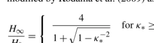
For comparison purposes the amplification ratio,H∞/H0, predicted by Miles (1977) for solitary waves is calculated us-ing the interaction parameter,κ∗=tanθ0/(
√
3H0/ hcosθ0), modified by Kodama et al. (2009) as
H∞ H0 = 4 1+ q 1−κ∗−2
forκ∗≥1,
(1+κ∗)2 forκ∗<1.
(17)
The interaction parameterκ∗ is inversely proportional to √
H0/ h, while the parameterKis proportional to(kH0)2. To properly compare the nonlinear effects on the generation of stem waves a new parameterK∗for Stokes waves is proposed as
K∗=γ K−1/4∼1/ p
kH0, (18)
Figure 13.Comparison of calculated and measured stem angle αas a function of nonlinear parameterK. Dashed curves represent the calculated values using Yue and Mei (1980), solid curves are the calculated values using Eq. (12), symbols are measured data. Red and blue colors are forθ0=10 and 20◦, respectively.
Figure 14.Comparison of amplification ratios,H∞/H0, as a function of nonlinear parameterκ∗for solitary waves andK∗for Stokes waves. Black solid curve represents the Miles’ solution for solitary waves, red and blue solid curves denote the calculated values for Stokes waves forθ0=10◦and 20◦, respectively. Symbols are measured data for Stokes waves.
solid line denotes the amplification ratio calculated using Eq. (17) for solitary waves, while red and blue solid lines represents the amplification ratios obtained from numerical computations for the Stokes waves. The symbols denote the measured amplification ratios. As shown in the figure the am-plification ratios for the Stokes waves are much smaller than those of solitary waves. And the maximum amplification ra-tio for the Stokes waves is 2, while that of solitary waves is 4. This indicates that the intensity of the resonant interaction between the incident and the reflected waves is much weaker
than the case of the solitary waves due to strong frequency dispersion.
6 Conclusions
also obtained and compared with the measured data. The re-sults obtained from this study are summarized as follows.
1. For small-amplitude waves, the wave height along the wall shows slowly varying undulations with the average value ofH /H0=2.0. The maximum value of an undu-lation is approximately H /H0≈2.3, and the distance from the tip to the location of maximum wave height de-creases with increasing angle of incidence. Normalized wave heights perpendicular to the wall show a standing wave pattern. In particular, the wave height distributions for these small-amplitude waves show no sign of stem waves. Both numerical and linear analytical solutions agree reasonably well with measured wave heights. 2. As the amplitude of incident waves increases, the
un-dulation intensity decreases along the wall. For larger-amplitude waves with smaller angle of incidence, i.e., larger K values, the measurements show clear stem waves along the wall. Numerical simulation results are in good agreement with the results of laboratory experi-ments, while the analytical solution gives no stem wave, because it is linear.
3. Stem waves can develop when the nonlinear parameter
K is greater than approximately 0.46. As the nonlinear parameterK increases, the normalized stem height de-creases and the stem width inde-creases.
4. The resonant interactions between the incident and re-flected waves predicted for solitary waves are not ob-served for the periodic Stokes waves. The amplification ratios along the wall do not exceed 2 for the case of Stokes waves, while those can reach 4-fold for the soli-tary waves.
5. The existence and the properties of stem waves for si-nusoidal waves found theoretically via numerical sim-ulations are favorably supported by the physical exper-iments conducted in this study. Experimental data ob-tained in this study can be used as a useful tool to verify nonlinear dispersive wave numerical models.
Data availability. All figures for the experimental and calculated data are presented in this supplement.
Supplement. The supplement related to this article is available online at: https://doi.org/10.5194/npg-25-521-2018-supplement.
Competing interests. The authors declare that they have no conflict of interest.
Acknowledgements. This study was performed by a project of “In-vestigation of large swell waves and rip currents and development of the disaster response system (No. 20140057)” sponsored by the Ministry of Oceans and Fisheries of Korea.
Edited by: Victor Shrira
Reviewed by: Tarmo Soomere and four anonymous referees
References
Berger, U. and Kohlhase, S.: Mach-reflection as a diffraction prob-lem, Proc. 15th Conf. Coastal Eng., Honolulu, Hawaii, July 1976, 796–814, 1976.
Chen, H. S.: Combined reflection and diffraction by a vertical wedge, Tech. Rep. CERC 87-16, US Army Corps of Engrs. (US-ACE) Wtrwy. Experiment Station, Vicksburg, Miss., USA, 1987. Gidel, F., Bokhove, O., and Kalogirou, A.: Variational modelling of extreme waves through oblique interaction of solitary waves: application to Mach reflection, Nonlin. Processes Geophys., 24, 43–60, https://doi.org/10.5194/npg-24-43-2017, 2017.
Kadomtsev, B. and Petviashvili, V.: On the stability of solitary waves in weakly dispersing media, Sov. Phys. Dokl, 539–541, 1970.
Kirby, J. T.: Large-angle parabolic equation methods, Proceedings of the 20th International Conference on Coastal Engineering, Taipei, November, 410–424, 1986.
Kirby, J. T. and Dalrymple, R. A.: Combined refraction/diffraction model REF/DIF 1, Version 3.0: Documentation and User’s Man-ual, Center for Applied Coastal Research, Department of Civil Engineering, University of Delaware, Delaware, USA, 2002. Kodama, Y.: KP solitons in shallow water, J. Phys. A: Mathematical
and Theoretical, 43, 434–484, 2010.
Kodama, Y., Oikawa, M., and Tsuji, H.: Soliton solutions of the KP equation with V-shape initial waves, J. Phys. A, 42, 312–321, 2009.
Lee, J. and Kim, Y.: Numerical analysis of stem waves along a ver-tical wall, J. Coast. Res., 1101–1105, 2007.
Lee, J. I. and Yoon, S. B.: Hydraulic and numerical experiments of stem waves along a vertical wall, J. Korean Soc. Civil Eng., 26, 405–412, 2006.
Lee, J.-I., Kim, Y.-T., and Cho. Y.-S.: Hydraulic model test for stem waves along vertical wall under regular wave actions, Proc. of Annual Conf. of Korean Society of Civil Engineers, October 2003, Daegu, Korea, 4939–4943, 2003.
Le Mehaute, B.: An introduction to hydrodynamics and water waves, Springer, New York, 525 pp., 1976.
Li, W., Yeh, H., and Kodama, Y.: On the Mach reflection of a soli-tary wave: revisited, J. Fluid Mech., 672, 326–357, 2011. Liu, P. L. F. and Yoon, S. B.: Stem waves along a depth
discontinu-ity, J.Geophys. Res.-Oceans, 91, 3979-3982, 1986.
Melville, W.: On the mach reflexion of a solitary wave, J. Fluid Mech., 98, 285–297, 1980.
Mei, C. C., Stiassnie, M., and Yue, D. K.-P.: Theory and applica-tions of ocean surface waves: Part 1: Linear aspects Part 2: Non-linear aspects, World Scientific, Singapore, 809–816, 2005. Miles, J. W.: Obliquely interacting solitary waves, J. Fluid Mech.,
Miles, J. W.: Resonantly interacting solitary waves, J. Fluid Mech., 79, 171–179, 1977b.
Nicholls, D. P.: On hexagonal gravity water waves, Math. Comp. Sim., 55, 567–575, 2001.
Perroud, P. H.: The solitary wave reflection along a straight vertical wall at oblique incidence, IER Report. 99-3, 93, University of California, Berkeley, California, USA, 1957.
Postacchini, M., Brocchini, M., and Soldini, L.: Vorticity generation due to cross-sea, J. Fluid Mech., 744, 286–309, 2014.
Soomere, T.: Interaction of Kadomtsev-Petviashvili solitons with unequal amplitudes, Phys. Lett. A, 332, 74–81, 2004.
Suh, K. D., Park, W. S., and Park, B. S.: Separation of incident and reflected waves in wave–current flumes, Coast. Eng., 43, 149– 159, 2001.
Yoon, S. B. and Liu, P. L.-F.: Stem waves along breakwater, J. wa-terway, Port Coast. Ocean Eng., 115, 635–648, 1989.