https://doi.org/10.5194/cp-15-893-2019
© Author(s) 2019. This work is distributed under the Creative Commons Attribution 4.0 License.
Varying regional
δ
18
O–temperature relationship in
high-resolution stable water isotopes from east Greenland
Christian Holme1, Vasileios Gkinis1, Mika Lanzky1,2, Valerie Morris3, Martin Olesen4, Abigail Thayer3, Bruce H. Vaughn3, and Bo M. Vinther1
1Centre for Ice and Climate, The Niels Bohr Institute, University of Copenhagen, Copenhagen, Denmark 2Department of Geosciences, University of Oslo, Oslo, Norway
3Institute of Arctic and Alpine Research, University of Colorado Boulder, Boulder, Colorado, USA 4Danish Climate Centre, Danish Meteorological Institute, Copenhagen, Denmark
Correspondence:Christian Holme (christian.holme@nbi.ku.dk)
Received: 11 December 2018 – Discussion started: 13 December 2018 Accepted: 29 April 2019 – Published: 16 May 2019
Abstract.This study examines the stable water isotope sig-nal (δ18O) of three ice cores drilled on the Renland penin-sula (east Greenland coast). While ice core δ18O measure-ments qualitatively are a measure of the local temperature history, theδ18O variability in precipitation actually reflects the integrated hydrological activity that the deposited ice experienced from the evaporation source to the condensa-tion site. Thus, as Renland is located next to fluctuating sea ice cover, the transfer function used to infer past tempera-tures from the δ18O variability is potentially influenced by variations in the local moisture conditions. The objective of this study is therefore to evaluate theδ18O variability of ice cores drilled on Renland and examine the amount of the signal that can be attributed to regional temperature varia-tions. In the analysis, three ice cores are utilized to create stacked summer, winter and annually averagedδ18O signals (1801–2014 CE). The imprint of temperature onδ18O is first examined by correlating the δ18O stacks with instrumental temperature records from east Greenland (1895–2014 CE) and Iceland (1830–2014 CE) and with the regional climate model HIRHAM5 (1980–2014 CE). The results show that the δ18O variability correlates with regional temperatures on both a seasonal and an annual scale between 1910 and 2014, while δ18O is uncorrelated with Iceland temperatures between 1830 and 1909. Our analysis indicates that the un-stable regionalδ18O–temperature correlation does not result from changes in weather patterns through strengthening and weakening of the North Atlantic Oscillation. Instead, the results imply that the varying δ18O–temperature relation is
connected with the volume flux of sea ice exported through Fram Strait (and south along the coast of east Greenland). Notably, theδ18O variability only reflects the variations in regional temperature when the temperature anomaly is posi-tive and the sea ice export anomaly is negaposi-tive. It is hypoth-esized that this could be caused by a larger sea ice volume flux during cold years which suppresses the Iceland temper-ature signtemper-ature in the Renlandδ18O signal. However, more isotope-enabled modeling studies with emphasis on coastal ice caps are needed in order to quantify the mechanisms be-hind this observation. As the amount of Renlandδ18O vari-ability that reflects regional temperature varies with time, the results have implications for studies performing regression-basedδ18O–temperature reconstructions based on ice cores drilled in the vicinity of a fluctuating sea ice cover.
1 Introduction
of precipitation on an ice cap. Hence, by drilling ice cores at polar sites such as Antarctica and Greenland, it is possi-ble to access past temperatures imprinted on the δ18O sig-nal. Several studies have examined the relation between tem-perature and ice core δ18O, and its linear or quadratic re-lationship has regularly been used as a transfer function to infer past temperature (Jouzel and Merlivat, 1984; Johnsen et al., 1989, 2001; Jouzel et al., 1997; Ekaykin et al., 2017). While it is evident that δ18O and temperature covary, the δ18O signal is also affected by changes in sea ice and at-mospheric circulation (Noone and Simmonds, 2004; Steig et al., 2013). Changes in regional quasi-stationary modes of climate variability such as the North Atlantic Oscillation can modulate global atmospheric circulation patterns (e.g., pre-cipitation patterns) which affect theδ18O variability. Addi-tionally, changes in sea ice extent affect the local moisture conditions, which particularly influence the coastal precipi-tatedδ18O variability (Bromwich and Weaver, 1983; Noone and Simmonds, 2004). Such variations have implications for a simple regression-based reconstruction of temperature from δ18O as the variability patterns between the ice core isotope signal and the oscillation modes and sea ice extent can have varied in strength back in time. Furthermore, in studies that analyze the relationship between polar precipi-tatedδ18O and temperature, the temperature record is often substantially shorter than the δ18O series. While this is in-evitable when performing temperature reconstructions, uti-lizing a short temperature record complicates the possibility of verifying whether the estimated δ18O–temperature rela-tion is stable with time.
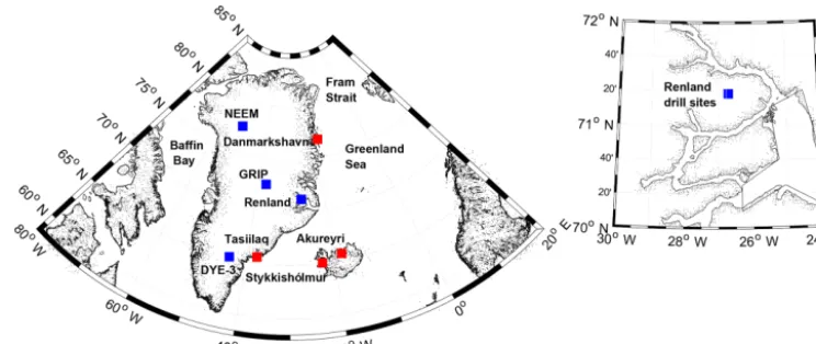
The aim of this study is to examine how much of the δ18O variability (1801–2014 CE) from a stack of ice cores drilled on the Renland peninsula, eastern Greenland, can be attributed to temperature variations (map in Fig. 1). In the analysis, seasonally averaged δ18O time series have been compared with regional temperatures through instrumen-tal temperature records from the coasts of east Greenland (1895–2014 CE) and Iceland (1830–2014 CE) and the re-gional atmospheric climate model HIRHAM5 2 m tempera-ture output (1980–2014 CE). Theδ18O signal is divided into its seasonal components as it potentially improves the recon-struction of variability in weather regimes and past temper-atures (Vinther et al., 2003b, 2010; Zheng et al., 2018). As Renland is located on the coast, its hydrological conditions are connected with the sea ice that is transported south an-nually along the coast of east Greenland. A relatively small loss in regional sea ice extent (≈ 10 % or less) has previously been found to influence local Greenland moisture source wa-ter vapor, which is traceable in the corresponding ice core deuterium excess values (Klein and Welker, 2016). The deu-terium excess signal (dxs=δD−8·δ18O; Dansgaard, 1964) contains information about the kinetic fractionation occur-ring when moisture evaporates from the ocean surface and the ice core dxs has been found to correlate with relative humidity and sea surface temperature at the source region
(Jouzel and Merlivat, 1984; Johnsen et al., 1989). Thus, be-sides investigating the regionalδ18O–temperature relation-ship, this study examines if changes in the Arctic sea ice ex-tent can be detected in the Renland stable water isotopes.
2 The ice cores
The Renland ice cap has an area of 1200 km2 with an av-erage ice thickness of a few hundred meters. It is separated from the main Greenlandic ice sheet as a small peninsula on the east coast of Greenland (map in Fig. 1). The ice cap ex-periences a high annual accumulation rate of around 0.47 m ice yr−1with an annual surface temperature of−18◦C. Ren-land has probably never been overridden by the inRen-land ice as it is surrounded by deep branches of the Scoresbysund Fjord which effectively drains the inland ice (Johnsen et al., 1992). Additionally, the small width of the ice cap, which is con-strained by the surrounding mountains, prevents the ice ele-vation from significantly increasing from present-day height. As a result, the ice cap has not experienced any ice sheet elevation changes for the past 8000 years (except for slight uplift due to isostatic rebound) (Vinther et al., 2009). This implies that lapse-rate-controlled temperature variations re-sulting from a varying ice sheet thickness will be negligible. This study utilizes three ice cores drilled on Renland in the analyses (Table 1). Two cores were drilled next to each other in the year 1988 (main (M) and shallow (S) cores), while the third was drilled approximately 2 km away in 2015 as part of the REnland ice CAP project (RECAP). The 1988 M and RE-CAP cores extend over the past 120 ka, while the 1988 S core only covers the time back to the year 1801. Despite two cores covering the past interglacial and glacial period, the study fo-cuses on the period 1801–2014 CE where three overlapping ice core records and instrumental temperature recordings are available. Moreover, the separation of the summer and win-ter signals is betwin-ter facilitated when the annual layers are not obliterated due to diffusion and ice thinning.
Figure 1.Locations of ice core drill sites (blue squares) and the instrumental temperature records (red squares).
Table 1.The subset of the three ice cores used in this study: processing information, analysis and coordinates.
Cores Coordinates Time span Depth span Meas. Resolution Analysis
RECAP 71◦1801800N, 26◦4302400W; 2315 m a.s.l. 1801–2014 111.7 m δ18O,δD 0.5 cm CFA-L2130 1988 M 71◦1801700N, 26◦4302400W; 2340 m a.s.l. 1801–1987 92.5 m δ18O 5.0 cm IRMS 1988 S 71◦1801700N, 26◦4302400W; 2340 m a.s.l. 1801–1987 91.6 m δ18O 5.0 cm IRMS
3 Diffusion correction
Firn diffusion dampens the annual oscillations in the δ18O data. This takes place while firn (snow that survived a season) is transformed into ice in the top 60–80 m of the ice sheet. During this densification process, air in the open porous firn is interconnnected, which enables the stable water isotopes in the firn air to mix with the snow grains (Johnsen, 1977). This molecular diffusion process makes theδ18O sig-nal become increasingly more smooth with depth until pore close-off. The firn diffusion of stable water isotopes imposes two challenges on the analysis presented in this study. First, the diffusion of the annual oscillations creates artificial trends in summer and winter season time series of δ18O (Vinther et al., 2010). Secondly, it introduces a bias when compar-ing the ice cores drilled in 1988 with the ice core drilled in 2015. For instance, theδ18O signal representing the year 1987 has only experienced 1 year of firn diffusion in the 1988 ice cores, while it has experienced 28 years of firn diffusion in the 2015 core. Theδ18O signal for overlapping years will therefore be more attenuated in the 2015 core.
As this study compares the seasonally averagedδ18O sig-nals of three ice cores drilled in different years, it is nec-essary to ensure that each δ18O record has the same firn diffusive properties with depth. This is typically achieved by correcting each δ18O record such that the effect of in-creasing smoothing with depth is removed by deconvolving the measuredδ18O signal to restore the originally deposited signal. However, Renland frequently experiences summer melting which causes steep isotopic gradients in the firn.
Such high-frequency gradients complicate a deconvolution of the measuredδ18O signal (Cuffey and Steig, 1998; Vinther et al., 2010). Instead, this study forward-diffuses the three δ18O records with depth such that eachδ18O series has been influenced by the same amount of firn diffusion. Diffusion of stable water isotopes is typically described by the diffusion length (σ), which is the average vertical displacement of a water molecule (units in meters). Thus, theδ18O series are forward-diffused (δ18Ofd) such that each record has the same σ with depth. Despite such a smoothing procedure slightly mixing the summer and winter signals, a distinction of the seasonal components is still possible due to Renland’s thick annual layers greatly exceeding the diffusion length.
The procedure below outlines in three steps how this was done separately for the 2015, 1988 M and 1988 S cores.
Step 1.First, the amount of diffusion that the measured δ18O signal already has experienced with depth is computed through the diffusion length’s density dependence (for origin, see Gkinis et al., 2014; Holme et al., 2018):
σ2(ρ)= 1 ρ2
ρ
Z
ρo 2ρ2
dρ
dt −1
D(ρ) dρ, (1)
model to density measurements from the drill sites. From Eq. (1), it is possible to calculate the diffusion length that each layer has experienced (σ2(ρ)) (Fig. C1a).
Step 2. Eq. (1) can be used to calculate the auxiliary diffusion needed to transform a δ18O record into having a uniform diffusion length independent of depth. An auxil-iary diffusion (σ2(ρ)aux) is calculated as the difference be-tween the final diffusion length at the pore close-off density (σ2(ρpc=804.3 kg m−3)) and the diffusion length at a given layer in meters of ice-equivalent depth:
σ2(ρ)aux=
ρpc
ρi 2
σ2(ρpc)−
ρ(z)
ρi 2
σ2(ρ) !
·
ρi ρ(z)
2 ,
(2)
where the fractionρi/ρ(z) ultimately is multiplied onto the auxiliary diffusion length in order to transform theσ2(ρ)aux from representing ice-equivalent depth to density-equivalent depth (as the annual oscillations are squeezed during firn compaction). Using Eq. (2), an auxiliary diffusion profile with respect to density (and thus depth) is calculated for an ice core (Fig. C1a).
Step 3.Forward diffusion is then simulated through a con-volution of the measured data (δ18Omeas) with a Gaussian fil-ter (G) with a standard deviation equal the auxiliary diffusion length as this is mathematically equivalent to firn diffusion (Johnsen, 1977):
δ18Ofd(z)=δ18Omeas∗G, (3)
where
G(z)= 1 σaux
√ 2πe
−z2/2σaux2
. (4)
As the auxiliary diffusion length decreases with depth, the width of the Gaussian filter changes accordingly. Thus, the convolution (using the σaux for the corresponding depth) is applied to a moving 2 m section which is shifted in small steps equal to the sampling interval. For each convolved data section, only the midpoint of the sliding window is retained as the new forward-diffusedδ18Ofd value. In order to avoid tail problems when diffusing the top 2 m measurements, the δ18Omeasdata were extended by using its prediction filter co-efficients estimated from a maximum entropy method algo-rithm by Andersen (1974). This assumes that the extended series has the same spectral properties as the original series. After applying this smoothing routine to the entire record, a δ18Ofd series with constant σ is obtained. A comparison betweenδ18Ofdandδ18Omeasis shown in Fig. C1.
4 Chronology
It is important to ensure that the chronologies of the three ice cores are synchronous before comparing theδ18O variability.
The two cores drilled in 1988 were manually dated by count-ing the summer maxima and winter minima in theδ18O se-ries and verified by identifying signals of volcanic erup-tions in the electrical conductivity measurements (Vinther et al., 2003b, 2010). For the 2015 RECAP core, the period 1801–2007 was dated with the annual layer algorithm (Strati-Counter) presented in Winstrup et al. (2012) and the years 2007–2014 were manually counted similar to the 1988 cores (the RECAP chronology is presented in Simonsen et al., 2018). The annual layer algorithm uses signals in the ice core that all have annual oscillations or peaks such as the chemical impurities (Na+, Ca, SO24−and NH+4), electrical conductiv-ity and stable water isotopes. Even though the model auto-matically counts years, the chronology is still restricted by the same volcanic eruptions as in the 1988 cores. The model marks a year when Na+ has a peak, which indicates win-ter. Na+ is a result of the transport of salt from the ocean, and it peaks during winter due to the strong winds during the fall. As the timing of this winter peak might not be simi-lar to the timing of theδ18O series’ winter minima (used for the 1988 cores), this study has tuned the RECAP dating pre-sented Simonsen et al. (2018) slightly. For each year, this is done by tuning the timing of the summer and winter in the dated RECAP record to match the maximum and minimum of theδ18O series. The chronology is only shifted a maxi-mum of a few months, and it is only changed within a given year. This ensures that the modified dating profile remains consistent with the original chronology, while it facilitates an optimal comparison between the manually dated and the automatically dated stable water isotopes profiles.
In order to analyze the seasonal signals of theδ18O se-ries, we need to distinguish between snow deposited dur-ing summer and winter. Under the assumption thatδ18O and temperature extremes in the Greenland region occur simul-taneously, Vinther et al. (2010) found it best to define the summer and winter seasons such that they each contain 50 % of the annual accumulation. Besides maximizing the amount of utilized data, this definition ensures that the winter and summer signals contain no overlapping data. This study has therefore defined the summer and winter seasons similarly to Vinther et al. (2010). The summer, winter and annually aver-agedδ18O data used in this study are thus seasonal or annual averages of the forward-diffusedδ18O series.
5 δ18Ovariability on Renland
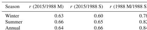
coeffi-Table 2.Correlation coefficients (r) calculated for different combi-nations ofδ18O records for the period 1801–1987 (p <0.05).
Season r(2015/1988 M) r(2015/1988 S) r(1988 M/1988 S) Winter 0.63 0.60 0.78 Summer 0.66 0.65 0.82 Annual 0.64 0.66 0.84
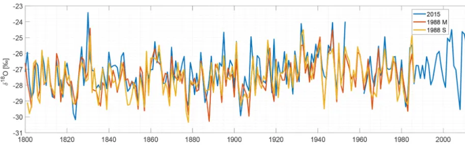
cient calculations throughout this study, the level of signifi-cance is estimated based on a Monte Carlo routine described in Appendix B. From the results displayed in Table 2, it is evident that the lowest correlation coefficients are found for the winter-averaged data with values ranging from 0.60 to 0.78, while the summer- and annually averaged signals have higher values ranging from approximately 0.64 to 0.84. The high correlation coefficients indicate that there is a strong lin-ear relationship between theδ18O records. This is further il-lustrated by the visual covariation of the annually averaged δ18O records in Fig. 2. In all instances, the highest correla-tions are found when correlating the two ice cores drilled in 1988. This might be attributed to the use of a similar dat-ing method and their close proximity. Nonetheless, all the presented ice cores correlated significantly during the 1801– 1987 period.
The δ18O variability can be further analyzed by examin-ing the mean sexamin-ingle series SNR which provides an insight into the amount of signal and noise in theδ18O series (Fisher et al., 1985). Noise can originate from depositional effects such as wind shuffling of snow and melt layers and from dat-ing uncertainties (±1 year) in between the three cores. By averagingn(3) overlapping ice core data records, the mean single series SNR is calculated by comparing the variance of an averaged record (VARs) with the mean of the variances (VAR) for the n individual records (Johnsen et al., 1997; Vinther et al., 2006):
SNR= VARs −VAR
n VAR−VARs
. (5)
Alternatively, a recent study by Münch and Laepple (2018) introduced a new way of calculating timescale-dependent SNR values, which provides a basis for interpreting noise across timescales. The SNR results are shown in Table 3. Similar to the high correlation, it is evident that merging the two 1988 records results in the highest SNR values. More-over, the summer-averaged signal has a higher SNR com-pared to the winter-averaged signal, which probably is a con-sequence of winters having more windy conditions that gen-erate the redeposition of snow. A similar pattern has pre-viously been found for the seasonal isotopes of GRIP ice core (n=5; SNR summer: 0.70; winter: 0.51), Dye-3 ice core (n=2; SNR summer: 1.73; winter: 1.56) and NEEM ice core (n=4; SNR summer: 1.28; winter: 0.64) (map in Fig. 1) (Vinther, 2003a; Zheng et al., 2018). This compari-son also shows that the SNR values of the three Renland ice
Table 3.Mean signal-to-noise variance ratios calculated for the summer, winter and annually averaged data using two and three cores in the period 1801–1987.
Merged cores SNR winter SNR summer SNR annual
1988 M, 2015 1.65 1.73 1.73 1988 M, 1988 S 3.53 4.46 5.05 1988 M, 1988 S, 2015 2.01 2.36 2.43
cores are high compared to GRIP, Dye-3 and NEEM which likely can be attributed to a combination of a high accumu-lation rate and a good cross-dating between the compared cores.
From this analysis, the study can comment on two things. First, the two 1988 cores have the most robust common sig-nal of all the tested combinations. As this was for two adja-cently drilled ice cores, utilizing all three records still results in a larger spatial atmospheric representativeness of the re-gion. Secondly, the high SNR and correlation coefficients im-ply that the chronologies from the annual layer detection al-gorithm and the manual counting are consistent. This has im-plications for future ice core science as manual layer count-ing can be a slow and inefficient procedure. Thus, manual counting can effectively be replaced with the StratiCounter software by Winstrup et al. (2012) for ice cores, where sev-eral datasets that contain observable annual peaks or oscilla-tions are available.
The high combined SNR values and correlation coeffi-cients indicate that it is beneficial to combine the time series into a stackedδ18O record. We choose to employ all three ice cores as that increases the spatial representativeness of δ18O, while it provides water isotopic variability for the years 1988–2014. A stacked record is typically created by averag-ing the time series but the time span 1801–2014 consists of an inhomogeneous amount of data records as only the RE-CAP core contains data in the 1988–2014 period, while it also has a gap between 1954 and 1961 due to missing ice samples. Thus, it is important to implement a variance cor-rection in order to avoid bias issues when averaging time se-ries with nonuniform length (Osborn et al., 1997; Jones et al., 2001). This variance correction (c) can be expressed directly through the SNR values in Table 3 and the number of records (m) used in the averaging for the given year (derivation can be found in Vinther et al., 2006):
c= s
SNR
SNR+1
m
. (6)
Figure 2.Annually averagedδ18O for the RECAP 2015 (blue), 1988 M (red) and 1988 S (yellow) cores with age.
year:
δ18Oavr=c· 1 m
m
X
i=1
δ18OSDi. (7)
The amplitude and variability of the original δ18O series are then restored by using the average variance (VAR) and the average (δ18O) of the three time series (from the period where the time series were standardized):
δ18Ostack=δ18Oavr· p
VAR+δ18O. (8)
Figure 3 shows the summer, winter and annual δ18Ostack series for the period 1801–2014. In the figure, a 5-year mov-ing average has been applied to the stacked records in order to filter out any remaining high-frequency noise variability. From the figure, it is evident that the summer-averaged nal is less depleted than the annual and winter-averaged sig-nals. Moreover, the summer signal has the largest trend in δ18O with an increase of 0.54 ‰ per century, while the win-ter and annually averaged data show lower increases of, re-spectively, 0.24 ‰ per century and 0.37 ‰ per century. The amount of variability that correlates with temperature will be examined in Sect. 6.
6 The temperature signature inδ18O
6.1 Correlation with instrumental temperature records The relationship between Renland δ18O variability and temperature is first investigated by comparing the stacked δ18O series with instrumental temperature records. This study uses the nearest and longest temperature recordings from Greenland (Tasiilaq and Danmarkshavn) and Iceland (Akureyri and Stykkishólmur) – locations are shown in Fig. 1. The Greenland temperature records are available from the Danish Meteorological Institute (2018) and the Iceland temperatures are available from the Icelandic Met Office (2018). For the temperature measurements, the seasons have
been defined similarly to Vinther et al. (2010) with summer extending from May to October and winter from November to April. Figure 4 shows the annually averagedδ18O stack to-gether with the annually averaged temperature measurements (winter and summer averages are shown in Figs. C2 and C3). Visually, the past 100 years of summer, winter and annually averagedδ18O signals of Renland covary with the regional temperature. However, the years 1830–1910 show periods with both anticorrelation and correlation. Besides the visual covariation, correlation coefficients between the temperature recordings and theδ18O stacks are calculated and shown in Table 4. The correlations with the winter-averaged data are in general the lowest, while annual and summer signals have similar high correlations at all the sites. The best correlation with the Renlandδ18O signal is found for the annual aver-ages at Tasiilaq (r=0.50). Additionally, applying a 5-year moving mean on theδ18O and temperature series increases all the correlations (i.e., the Tasiilaq correlation coefficient increases tor=0.72).
Figure 3.Summer (red), winter (blue) and annually averaged (green)δ18O stacks together with their corresponding linear trends (black lines) for the period 1801–2014. A moving average of 5 years has been applied to all the time series. For the unfiltered series, the reader is referred to Figs. 4, C2 and C3.
Figure 4.Annually averagedδ18O and temperature series. For visualization, the time series have been standardized and shifted vertically. The black curves represent a moving average of 5 years.
the high correlations in the 1910–2014 period. This could explain why the highest δ18O–temperature correlation was found at Tasiilaq as it only extended back to 1895. Conse-quently, the regionalδ18O–temperature relationship between Renland isotopes and the Iceland temperature record is not constant through time. While it remains unknown if the tem-perature on Iceland and Renland was similar between 1830 and 1909, it is certain that the Renlandδ18O variability does not represent the temperature variability in Iceland in the studied period. Thus, even though theδ18O variability prob-ably reflects the local temperature on Renland, the results show that the spatial extent of this δ18O–temperature rela-tionship was different in the 1830–1909 period.
6.2 Correlation with the HIRHAM52m temperature output
Table 4.Correlation coefficients between theδ18O stack and instrumental temperature records (p <0.05) both at a 1-year resolution and with a 5-year moving mean applied (in bold).
Record Stykkishólmur Akureyri Danmarkshavn Tasiilaq
Period 1830–2014 1931–2014 1951–2014 1895–2014 rwinter 0.29/0.51 0.30/0.56 0.21/0.51 0.41/0.64 rsummer 0.40/0.58 0.45/0.69 0.30/0.62 0.37/0.61 rannual 0.48/0.62 0.40/0.58 0.35/0.63 0.50/0.72
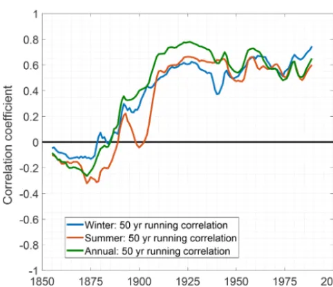
Figure 5.Running correlation of 50 years between the Stykkishól-mur temperature and theδ18O stack for winter (blue), summer (red) and annual averages (green). Both theδ18O and temperature data were first smoothed with a 5-year moving mean. Each year repre-sents the midpoint of the running window.
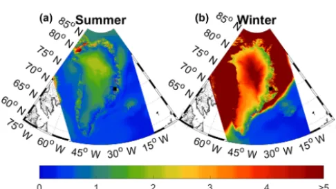
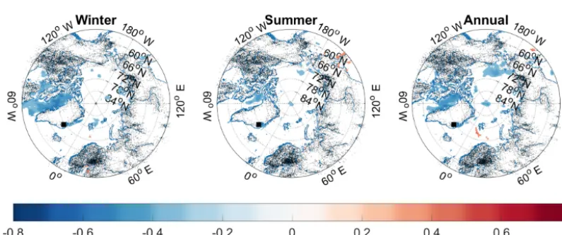
April, respectively. The RECAP core is used instead of the stacked record as the analysis is on data from the satellite era, which is minimally available in the 1988 cores. The cor-relation maps are shown in Fig. 6. The results show sig-nificant positive correlations between the winter signals of HIRHAM5 2 m temperature and the RECAP δ18O. More-over, the high correlations (r >0.5) that extend over most of Greenland, irrespectively of the ice divide, indicate that the winter temperature variability over Greenland is imprinted in the Renlandδ18O signal. Results furthermore show that there is no statistically significant correlation between δ18O and temperature east of Renland in areas regularly covered by sea ice. For the summer and annually averaged signals, the correlations are lower (r∼0.4–0.5) and they only cover the east coast region. This local spatial pattern is consistent with Vinther et al. (2010), who found that the summer-averaged δ18O data from different Greenlandic ice cores were less in-ternally coherent than the corresponding winter data. This could explain why the summerδ18O variability of the
RE-CAP core only correlates with the local temperatures on the coast of east Greenland. Moreover, the variance in summer-averaged temperatures over Greenland is very low, as shown in Fig. 7. The low variance is due to the HIRHAM5 sum-mer temperatures reaching a maxima just below 0◦C at places with constant ice cover. For instance, Fig. 8 shows the monthly averaged HIRHAM5 temperature from a grid point on Renland where it is evident that the monthly aver-aged temperature fluctuations during summer are very small. Thus, the small temperature fluctuations can limit the possi-bility of interpreting the spatial extent of summer and annual temperature variability imprinted in theδ18O signal.
All in all, these results support the correlations from Sect. 6.1 that were high between δ18O and temperature in the 1910–2014 period.
7 The North Atlantic Oscillation’s imprint onδ18O
A strengthening and weakening of, respectively, the low-pressure system over Iceland and high-low-pressure system over the Azores control both the direction and strength of west-erly winds and storm tracks over the North Atlantic. Fluctu-ations in the difference in atmospheric pressure at sea level between Iceland and the Azores is described by the North Atlantic Oscillation (NAO). Changes in the NAO has previ-ously been found to have an imprint on precipitation in west-ern Greenland (Appenzeller et al., 1999). Correspondingly, the winter isotope signal of west and south Greenland ice cores have previously been found to anticorrelate with the at-mospheric circulation changes from the NAO (Vinther et al., 2003b, 2010). Despite Vinther et al. (2010) showing that ice cores drilled on the Greenland east coast revealed no connec-tion with the NAO, this study examines potential correlaconnec-tion in order to determine if changes in the NAO can be linked to the varyingδ18O–temperature relationship.
Figure 6.Figures showing the correlation between winter(a), summer(b)and annually(c)averaged RECAPδ18O and HIRHAM5 temper-atures. Only correlations withp <0.05 are shown.
Figure 7.Variances of the summer(a)and winter-averaged tem-peratures(b). A maximum variance of 5 (◦C)2is displayed in order to emphasize the small variance in the summer-averaged signal.
time). This study uses a slightly modified version of this NAO index by Vinther et al. (2003c), who improved the NAO record in the period 1821–1856 by using extra pressure se-ries.
The connection between the NAO index and seasonally (and annually) averaged δ18O stacks is examined by esti-mating their correlation. Correlation coefficients have been calculated on 5-year moving averages of the NAO and δ18O stacks and shown in Table 5 (the annual NAO record is plotted in Fig. 9). The level of significance is estimated based on a Monte Carlo routine described in Appendix B. In the complete 1821–2014 period, the summer, winter and annu-ally averaged NAO andδ18O data are uncorrelated with co-efficients of 0.01,−0.05 and 0.02, respectively. If we instead examine the time before and after theδ18O–temperature cor-relation terminated (the year 1909), the summer and annually averaged data yield positive correlations of 0.29 and 0.30 be-tween 1821 and 1909, while the winter and annually aver-aged data yield negative correlations of −0.25 and −0.22 between 1910 and 2014. Thus, there is a varying relation be-tween the NAO and theδ18O data, and the weakδ18O–NAO
anticorrelation coincides with a covaryingδ18O–temperature relation. However, the weak correlations during 1821–1909 imply that the NAO only can account for around 8 %–9 % of the correspondingδ18O variability. It therefore seems un-likely that strengthening and weakening of the NAO causes changes in theδ18O–temperature relation.
8 The impact of sea ice fluctuations on the stable water isotopes
8.1 Fram Strait sea ice export
In this section, it is investigated whether there is a connection between the Renlandδ18O variability and the sea ice export (SIE) through the Fram Strait (map in Fig. 1). Sea ice from the Arctic Ocean is exported southward through Fram Strait along the eastern coast of Greenland into the Greenland Sea. Fluctuations in this sea ice volume flux have a direct effect on the amount of open water located east and northeast of Renland. Asδ18O is an integrated signal of the hydrological activity along the moisture transport pathway from evapo-ration source to deposition, the open water which facilitates moist and mild climatic conditions will likely affect the iso-topic composition of the precipitation deposited on Renland. Essentially, besides the temperature dependence of isotopic fractionation during local condensation,δ18O contains infor-mation about the amount of water mass that is removed from the air during the poleward transport and the continuous con-tribution of local water mixing with the transported water mass (Noone and Simmonds, 2004).
Figure 8.Monthly averaged 2 m temperature from a grid point on Renland (blue curve) plotted together with the forward-diffusedδ18O from the RECAP ice core (red curve) and A6 snow pit core (green curve).
Table 5.Correlation coefficients between theδ18O stack and NAO index. Both time series have been smoothed with a 5-year moving mean. Only the numbers in bold are statistically significant (p <0.05).
Period 1821–1909 1910–2014 1821–2014
rwinter 0.15 (p=0.16) −0.25(p=0.01) −0.05 (p=0.52) rsummer 0.29(p <0.01) −0.15 (p=0.13) 0.01 (p=0.85) rannual 0.30(p <0.01) −0.22(p=0.02) 0.02 (p=0.82)
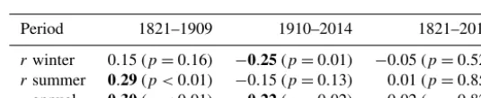
order to quantify any covariation of the records. For a mov-ing average of 5 years applied to the time series, there is an anticorrelation of−0.54 (p <0.01) between the annual SIE andδ18O, while there is no significant correlation between dxsand the SIE (r= −0.08). From the correlation analyses, it is clear thatδ18O anticorrelates with SIE, while it correlates with temperature (Sect. 6.1). In order to examine if these cor-relations apply simultaneously, correlation coefficients have been calculated on a 50-year running window. The level of significance is estimated based on a Monte Carlo routine de-scribed in Appendix B. The results are plotted in Fig. 10. In the past 100 years, the Stykkishólmur temperature record is found to correlate with Renland δ18O, while it (likeδ18O) anticorrelates with SIE through Fram Strait. This likely indi-cates that warm temperatures result in less sea ice that can be exported away from the Arctic Ocean (with less sea ice for-mation locally). However, this pattern ceases to exist prior to the early 1900s such that neither theδ18O signal or temper-ature share any correlation with the SIE. This synchronous decrease in correlation indicates that a lack of correlation betweenδ18O and temperature cannot be explained by dat-ing errors in the ice core chronologies. In addition, while we acknowledge that part of the missingδ18O–SIE correlation might be a consequence of the progressively decreasing sea ice data quality prior to 1900, we do not expect similar un-certainty with the instrumental temperature data. Thus, this indicates that the varying relationships are not solely an arti-fact of poor data quality. Furthermore, as discussed in Sect. 7 and shown as running correlations in Fig. 10, the varying
δ18O–temperature correlation cannot be a consequence of the NAO controlling theδ18O variability. Moreover, Fig. 10 also shows that changes in local moisture source regions are not traceable through thedxs–SIE correlation.
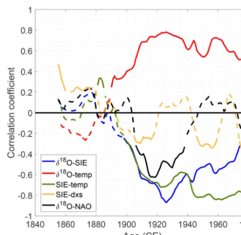
In order to examine the lacking δ18O–temperature cor-relation, the connection between the SIE anomaly and the δ18O–temperature relation is plotted in Fig. 11 (SIE anomaly is here defined as the deviation from the mean flux). As a 5-year moving mean has been applied to the time series, only every 5 points are used in the analysis. From the fig-ure, it is clear that in years when the temperature anomaly is positive (Tanom=T −Tmean), there is always a negative SIE anomaly and a high δ18O–temperature correlation of 0.83, whereas for Tanom<0 there is no δ18O–temperature correlation (r=0.02) which coincides with a combination of both positive and negative SIE anomalies. Besides show-ing that higher temperatures coincide with less sea ice be-ing transported south (likely due to an already lower ex-tent of sea ice), it appears that lower temperatures coincide with more fluctuations in the SIE, which possibly reduce the δ18O–temperature correlation. These results imply that the δ18O variability can be dominated by other climatic condi-tions such as SIE and does not only represent variacondi-tions in regional temperature for an extended period of time.
8.2 The sea ice edge in the Greenland Sea
Figure 9.Annually averagedδ18O stack (blue curve), Fram Strait SIE (yellow curve),dxs(green curve) and NAO index (black curve). A 5-year moving average has been applied to all the data.
record of seasonal SIL anomalies in the Greenland Sea from Divine and Dick (2006) to further examine the relation be-tweenδ18O and sea ice. The SIL anomaly (km) describes the advance and retreat of the ice edge position in the Greenland Sea (defined as the perpendicular distance from the mean edge to a given point). The SIL separates close pack ice (defined as concentrations greater than 30 %) from loose ice drift. Here, we only use data from the period 1850–2002 as it is has the highest density of data (we fill the gaps by linear interpolation). The record is based on historical observations of the ice edge and presents monthly averages for April, June and August where the sea ice extent are expected to experi-ence both its maximum (April) and its minimum (August). Only April and June data are used in this analysis as the data are too sparse for August.
This study compares the winter-averagedδ18O signal with the SIL data from April (maximum extent), the annually av-eragedδ18O with SIL data from June (intermediate extent) and the summer-averagedδ18O with the SIL data from June as they have approximately the same timing (all combina-tions are tested and the correlacombina-tions are displayed in Ta-ble C1). Similar to Sect. 8.1, correlations are calculated on a 50-year running window and displayed in Fig. 12. Ex-cept from a period of anticorrelation betweenδ18O and SIL (1890–1940), there exists no clear correlation pattern be-tween the Greenland Sea’s SIL and the Renlandδ18O signal. This is in contrast with the stronger connection between the Renlandδ18O signal and the SIE through Fram Strait. From Fig. 12, it is seen that the SIL and SIE data are uncorrelated
Figure 10.Running correlations of 50 years between Stykkishól-mur temperature and theδ18O stack (red), SIE and theδ18O stack (blue), SIE and Stykkishólmur temperature (green), theδ18O stack, and the NAO index (black) anddxs with SIE (yellow). The solid lines represent significant correlation (p <0.05), while the dashed lines are insignificantp >0.05. Each year represents the midpoint of the running window.
Figure 11.Annual temperature anomaly plotted with respect to an-nualδ18O anomaly, where colors indicate the strength of the Fram Strait sea ice export anomaly. A 5-year moving average has been ap-plied to all the time series but only every 5 points are displayed and used in the analysis. The solid black lines represents linear fits be-tweenδ18O and temperature for positive and negative temperature anomalies.
8.3 Sea ice concentration and sea surface temperature The Arctic sea ice concentration (SIC) data (fractional ice cover in percentage) from the ERA-Interim reanalysis (Dee et al., 2011) has been correlated with the RECAPδ18O and dxs series, and the results are shown in Figs. 13 and 14 (1980–2014). In the case of sea ice extent, summer refers to June-November and winter refers to December–May, while the seasonally averagedδ18O is defined similarly to Sect. 6.2 (summer: May–October; winter: November–April). In the case of dxs, only the annually averaged data are used as its seasonal components are smeared out after theδ18O and δD data have been forward-diffused. The results show a large patch of anticorrelation betweenδ18O and SIC in the Baffin Bay area (r≈ −0.4) outside west Greenland for both win-ter and annually averaged data. Presumably, this indicates that the climate at Renland is similar to the climate at Baf-fin Bay which controls the advance and retreat of the sea ice extent. A similar connection was found in Sect. 6.2, which showed that the winter-averagedδ18O signal correlated with temperatures all over Greenland, resembling the anticorrela-tions between NEEMδ18O and Baffin Bay SIC that have pre-viously been found (Steen-Larsen et al., 2011; Zheng et al., 2018). Moreover, the results are consistent with Faber et al. (2017), who found that changes in the Baffin Bay sea ice coverage can impact theδ18O precipitation over Greenland (by using an atmospheric general circulation model coupled with water isotopologue tracing (isoCAM3)). Furthermore, the analysis shows only a small patch of correlation between theδ18O series and the SIC south of Fram Strait. However, this is not necessarily inconsistent with the significant
anti-correlation presented in Sect. 8.1. Possibly, this nuance can be explained by the SIE representing the annual discharge of sea ice (ice volume flux), while the SIC represents the frac-tional ice cover in percentage (area).
The connection between the Renland stable water isotopes and the local climate conditions is further investigated by cor-relating the RECAPdxs signal with the Arctic SIC and sea surface temperature (SST). Figure 14 shows that there exist small patches of positive correlation patterns between thedxs signal and the SIC in the Arctic Ocean and south of Baffin Bay. As these areas are very small, it is difficult to evaluate the connection between the extent of SIC anddxsat Renland. Thedxs signal is further examined by checking if it reflects the local SST variability. This has been done by correlating thedxs signal with the SST data in the Arctic region from ERA-Interim data (1980–2014). From Fig. 14, it is evident that there barely exist patches with significant correlation. Thus, it is difficult to assess whether the RECAPdxsrecord directly reflects the local SST or SIC variability during the 1980–2014 period. More analysis on what controls the Ren-landdxssignal is needed in future research.
9 Discussion
distil-Figure 12.(a)Running correlations of 50 years between June SIL and summerδ18O (orange), April SIL and winterδ18O (red), June SIL and annualδ18O (blue), June SIL and Fram Strait SIE (green), and annualδ18O with Fram Strait SIE (purple).(b)Fram Strait SIE (blue) and Greenland Sea SIL (red) with 5- and 11-year moving means applied.
Figure 13.Maps showing the correlation coefficients between the ERA-Interim sea ice concentration and the RECAPδ18O data for the 1980–2014 period (p <0.05).
lation path and has risen in more altitude than that of the coastal region, further depleting theδ18O signal. In order to evaluate this hypothesis, more studies using isotope-enabled modeling are needed. The impact of changes in sea ice on the Arcticδ18O precipitation has previously been investigated by Faber et al. (2017), who found that theδ18O precipitation on Greenland only responded to perturbations of the Baffin Bay sea ice coverage. However, they used a horizontal resolution of∼1.4◦×1.4◦which barely resolved the Renland Ice Cap of∼1200 km2. Thus, a further examination of how changes in sea ice extent is connected with the coastal Greenlandic precipitation on a higher spatial resolution grid is essential in order to evaluate this hypothesis.
Alternatively, if the seasonal distribution of precipitation on Renland changed significantly prior to the 1910s, it could lead to a change in the relationship between theδ18O signals and temperature. While the dating resolution does not permit a direct assessment of such changes, we do observe that the difference between the summer and winterδ18O have in fact changed over the 1801–2014 period (Fig. 3).
tem-Figure 14.Maps showing thedxs-SST(a)anddxs-SIC correlation coefficients between annually averaged data from RECAP and ERA-Interim covering the 1980–2014 period (p <0.05).
peratures rather than an actual interconnection between Ren-landδ18O and Baffin Bay sea ice.
10 Conclusions
This study found that by quantifying the mean signal-to-noise variance ratios, a robust seasonal δ18O signal (1801– 2014) could be extracted by stacking three ice cores from Renland. This δ18O stack was correlated with instrumental temperature records from east Greenland and Iceland and with the HIRHAM5 2 m temperature output. Results showed that there were high correlations betweenδ18O and regional temperatures on both a seasonal and annual scale between 1910 and 2014. A similar anticorrelation was found between the δ18O stack and the amount of sea ice exported through Fram Strait. However, both correlations diminished in the 1830–1909 period. The results indicated that the varying re-gional temperature variability in the δ18O signal could not be explained by the North Atlantic Oscillation. Instead, the linear δ18O–temperature relation depended on whether the temperatures were warmer or colder than the temperature anomaly. Warm years were associated with a high correla-tion and accompanied by less sea ice transported south along the coast, while cold years were associated with zero correla-tion that accompanied a fluctuating amount of sea ice along the coast. These results implied that changes in the extent of open water outside Renland might affect the local mois-ture conditions. Hence, greater sea ice flux along the coast of Greenland may suppress the Iceland temperature signature in theδ18O signal; however, this was not confirmed by correla-tions betweendxs and sea surface temperature in the Arctic region. Thus, more high-resolution isotope-enabled
model-ing focused on the effect of Arctic sea ice on coastal precipi-tation are needed in order to quantify this process.
These results have implications for ice core temperature reconstructions based on the linear relationship between δ18O variability and local temperature records. For Renland, the linearδ18O–temperature relationship was unstable with time which implied that the annual-to-decadal variability of δ18O measured in an ice core could not be directly attributed to temperature variability. Similar conditions might apply for other ice cores drilled in the vicinity of a fluctuating sea ice cover. This reinforces the interpretation thatδ18O is an inte-grated signal of all the hydrological activity that a vapor mass experiences en route from the evaporation at the source to its condensation at the drill site.
Appendix A: Firn diffusivity
This study uses the firn diffusivity parameterization of Johnsen et al. (2000):
D(ρ)= m p Dai R T αiτ
1
ρ − 1 ρice
, (A1)
which depends on the molar weight of water (m), the satu-ration vapor pressure (p), diffusivity of water vapor (Dai), the molar gas constant (R), the site temperature (T), the ice– vapor fractionation factor (αi) and the firn air tortuosity (τ). Similar to Johnsen et al. (2000) and subsequently used in Si-monsen et al. (2011), Gkinis et al. (2014) and Holme et al. (2018), we used the following definitions which can be pa-rameterized through annual mean surface temperature, an-nual accumulation rate, surface pressure and density (ρ):
– saturation vapor pressure over ice (Pa) (Murphy and Koop, 2006):
p=exp
9.5504−5723.265 T
+3.530 ln(T)−0.0073T
; (A2)
– Dai – diffusivity of water vapor (for isotopologuei) in air (m2s−1). For the diffusivity of the abundant isotopo-logue water vaporDa(Hall and Pruppacher, 1976),
Da=2.1·10−5
T To
1.94 Po
P
, (A3)
withP0=1 atm,To=273.15 K, andP andT the am-bient pressure (atm) and temperature (K). Additionally from Merlivat and Jouzel (1979),Da2H=0.9755Daand Da18O=0.9723Da;
– R– molar gas constantR=8.3144 m3PaK−1mol−1;
– αi– ice–vapor fractionation factor. we use the formula-tions by Majoube (1970) and Merlivat and Nief (1967) forαsδ/Dvandαδs/18vO, respectively.
αIce/Vapor
2H/1H=0.9098 exp(16288/T2), (A4)
αIce/Vapor
18O/16O=0.9722 exp(11.839/T); (A5)
– τ – the firn tortuosity (Schwander et al., 1988):
1
τ =1−b·
ρ
ρice 2
ρ≤ρ√ice b, b
=1.3, (A7)
based on Eq. (A7),τ→ ∞forρ >804.3 kg m−3
Appendix B: Significance analysis
In this study, time series have often been smoothed with a 5-year moving mean before estimating their correlation. Po-tentially, this results in artificially improved correlation coef-ficients as a moving mean is a low-pass filter. It is therefore necessary to quantify the significance of the linear relation-ship (p value) by running a Monte Carlo simulation. This study tested significance by examining what correlation co-efficients we would estimate if we had randomly generated data instead of theδ18O signal (following the procedure pro-posed by Macias-Fauria et al., 2011). For simplicity, this sec-tion refers to the correlasec-tion betweenδ18O and temperature, while it applies equally for all types of time series.
Synthetic data are created by generating time series with the same power spectrum as theδ18O signal. This study uses a method outlined in Ebisuzaki (1977) that is based on a random resampling of theδ18O signal in the frequency do-main. The synthetic time series is then found by taking the inverse fast Fourier transform of the shuffled signal. This pro-cedure retains the same autocorrelation as the input time se-ries hereby mimicking the influence of a 5-year moving mean applied to data.
Appendix C: Figures and tables
Figure C1.(a) Modeled firn diffusion with depth (σ; blue) and calculated auxiliary diffusion length that should be applied to the measuredδ18O data (σaux; red). After the pore close-off (ρpc= 804.3 kg m−3),σaux=0 asσ just changes due to the compaction of firn.(b)The measuredδ18O data (blue) and the forward-diffused δ18O data (red) for the 1988 M core.
Figure C3.Summer-averagedδ18O and temperature series. For vi-sualization, the time series have been standardized and shifted ver-tically. The black curves represent a moving average of 5 years.
Figure C4.(a)Five-year moving average of the winter-averaged δ18O stack. (b) Five-year moving average of the December– January–February averaged southwest Greenland temperatures from Vinther et al. (2006).(c)50-year running correlations between δ18O and southwest Greenland (magenta) andδ18O and Stykkishól-mur (green). Each year represents the midpoint of the running win-dow. Solid lines are significant correlations and dashed lines are insignificant (p >0.05).
Table C1. Correlation coefficients for different combinations of sea ice line anomalies (SIL) versus Stykkishólmur temperature and δ18O for the period 1850–2000. The time series were first smoothed with a 5-year moving average. All the correlations are significant (p <0.05).
SIL April SIL Jun
δ18O winter −0.20 −0.19 δ18O summer −0.46 −0.48 δ18O annual −0.32 −0.32
Competing interests. The authors declare that they have no con-flict of interest.
Acknowledgements. The RECAP ice coring effort was financed by the Danish Research Council through a Sapere Aude grant, the NSF through the Division of Polar Programs, the Alfred We-gener Institute, and the European Research Council under the Eu-ropean Community’s Seventh Framework Programme (FP7/2007– 2013)/through the Ice2Ice project and the Early Human Impact project (267696). The authors acknowledge the support of the Dan-ish National Research Foundation through the Centre for Ice and Climate at the Niels Bohr Institute (Copenhagen, Denmark). We kindly thank Dmitry Divine and one anonymous reviewer whose thoughtful comments helped improve and clarify this paper.
Financial support. This research has been supported by the FP7 Ideas: European Research Council (grant no. ICE2ICE (610055)).
Review statement. This paper was edited by Elizabeth Thomas and reviewed by Dmitry Divine and one anonymous referee.
References
Andersen, N.: On the calculation of filter coefficients for maximum entropy spectral analysis, Geophysics, 39, 69–72, 1974. Appenzeller, C., Schwander, J., Sommer, S., and Stocker, T. F.: The
North Atlantic Oscillation and its imprint on precipitation and ice accumulation in Greenland, Geophys. Res. Lett., 25, 1939–1942, 1999.
Bromwich, D. H. and Weaver, C. J.: Latitudinal displacement from main moisture source controlsδ18O of snow in coastal Antarc-tica, Nature, 301, 145–147, 1983.
Christensen, O. B., Drews, M., Christensen, J. H., Dethloff, K., Ke-telsen, K., Hebestadt, I., and Rinke, A.: The HIRHAM Regional Climate Model Version 5, Technical report 06–17, Danish Cli-mate Centre, DMI, 2007.
Cuffey, K. M. and Steig, E. J.: Isotopic diffusion in polar firn: impli-cations for interpretation of seasonal climate parameters in ice-core records, with emphasis on central Greenland, J. Glaciol., 44, 273–284, 1998.
Danish Meteorological Institute: Greenland temperature records, available at: http://www.dmi.dk/laer-om/generelt/ dmi-publikationer/tekniske-rapporter/, last access: 1 Decem-ber 2018.
Dansgaard, W.: The18O-abundance in fresh water, Geochim. Cos-mochim. Ac., 6, 241–260, 1954.
Dansgaard, W.: Stable isotopes in precipitation, Tellus B, 16, 436– 468, 1964.
Dee, D. P., Uppala, S. M., Simmons, A., Berrisford, P., Poli, P., Kobayashi, S., Andrae, U., Balmaseda, M., Balsamo, G., Bauer, P., Bechtold P., Beljaars, A. C. M., van de Berg, L., Bidlot, J., Bormann, N., Delsol, C., Dragani, R., Fuentes, M., Geer, A. J., Haimberger, L., Healy, S. B., Hersbach, H., Hólm, E. V., Isak-sen, L., Kållberg, P., Köhler, M., Matricardi, M., McNally, A. P., Monge-Sanz, B. M., Morcrette, J.-J., Park, B.-K., Peubey, C., de
Rosnay, P., Tavolato, C., Thépaut, J.-N., and Vitart, F.: The ERA-Interim reanalysis: Configuration and performance of the data assimilation system, Q. J. Roy. Meteorol. Soc., 137, 553–597, 2011.
Divine, D. V. and Dick, C.: Historical variability of sea ice edge position in the Nordic Seas, J. Geophys. Res.-Ocean., 111, 1–14, 2006.
Ebisuzaki, W.: A method to estimate the statistical significance of a correlation when the data are serially correlated, J. Clim., 10, 2147–2153, 1977.
Ekaykin, A. A., Vladimirova, D. O., Lipenkov, V. Y., and Masson-Delmotte, V.: Climatic variability in Princess Elizabeth Land (East Antarctica) over the last 350 years, Clim. Past, 13, 61–71, https://doi.org/10.5194/cp-13-61-2017, 2017.
Epstein, S., Buchsbaum, R., Lowenstam, H., and Urey, H.: Carbonate-water isotopic temperature scale, Geol. Soc. Am. Bull., 62, 417–426, 1951.
Faber, A.-K., Møllesøe Vinther, B., Sjolte, J., and Anker Pedersen, R.: How does sea ice influence d18O of Arctic precipitation?, At-mos. Chem. Phys., 17, 5865–5876, https://doi.org/10.5194/acp-17-5865-2017, 2017.
Fisher, D. A., Reeh, N., and Clausen, H.: Stratigraphic noise in time series derived from ice cores, Ann. Glaciol., 7, 76–83, 1985. Gkinis, V., Simonsen, S. B., Buchardt, S. L., White, J. W. C., and
Vinther, B. M.: Water isotope diffusion rates from the NorthGRIP ice core for the last 16,000 years – glaciological and paleocli-matic implications, Earth Planet. Sc. Lett., 405, 132–141, 2014. Hall, W. D. and Pruppacher, H. R.: The Survival of Ice Particles
Falling from Cirrus Clouds in Subsaturated Air, J. Atmos. Sci., 33, 1995–2006, 1976.
Herron, M. M. and Langway, C. C.: Firn Densification: An Empiri-cial Model, J. Glaciol., 25, 373–385, 1980.
Holme, C., Gkinis, V., and Vinther, B. M.: Molecular diffusion of stable water isotopes in polar firn as a proxy for past tempera-tures, Geochem. Cosmochim. Ac., 225, 128–145, 2018. Holme, C.: Seasonally averagedδ18O ice core data (1801–2015 CE)
for Renland, Greenland, available at: http://www.iceandclimate. nbi.ku.dk/data/, last access: 15 May 2019.
Icelandic Met Office: Icelandic temperature records, available at: http://en.vedur.is/climatology/data/\T1\textbackslash#a, last ac-cess: 1 December 2018.
Johnsen, S., Clausen, H. B., Cuffey, K. M., Hoffmann, G., Schwan-der, J., and Creyts, T.: Diffusion of stable isotopes in polar firn and ice: the isotope effect in firn diffusion, Physics of Ice Core Records, 121–140, 2000.
Johnsen, S. J.: Stable Isotope Homogenization of Polar Firn and Ice, Isotopes and Impurities in Snow and Ice, 118, 210–219, 1977. Johnsen, S. J., Dansgaard, W., and White, J.: The origin of Arctic
precipitation under present and glacial conditions, Tellus B, 41, 452–468, 1989.
Johnsen, S. J., Clausen, H. B., Dansgaard, W., Gundestrup, N. S., Hansson, M., Jonsson, P., Steffensen, J. P., and Sveinbjornsdottir, A. E.: A “deep” ice core from East Greenland, Meddelelser om Groenland, Geoscience, 29, 3–22, 1992.
of possible Eemian climatic instability, J. Geophys. Res., 102, 26397–26410, https://doi.org/10.1029/97JC00167, 1997. Johnsen, S. J., Dahl-Jensen, D., Gundestrup, N., Steffensen, J. P.,
Clausen, H. B., Miller, H., Masson-Delmotte, V., Sveinbjorns-dottir, A. E., and White, J.: Oxygen isotope and palaeotemper-ature records from six Greenland ice-core stations: Camp Cen-tury, Dye-3, GRIP, GISP2, Renland and NorthGRIP, J. Quater-nary Sci., 16, 299–307, 2001.
Jones, P. D., Jonsson, T., and Wheeler, D.: Extension to the North Atlantic oscillation using early instrumental pressure observa-tions from Gibraltar and south-west Iceland, Int. J. Climatol., 17, 1433–1450, 1997.
Jones, P. D., Osborn, T. J., Briffa, K. R., Folland, C. K., Horton, E. B., Alexander, L. V., Parker, D. E., and Rayner, N. A.: Adjust-ing for samplAdjust-ing density in grid box land and ocean surface tem-perature time series, J. Geophys. Res., 106, 3371–3380, 2001. Jouzel, J. and Merlivat, L.: Deuterium and oxygen 18 in
precipita-tion: modeling of the isotopic effects during snow formation, J. Geophys. Res.-Atmos., 89, 11749–11759, 1984.
Jouzel, J., Alley, R. B., Cuffey, K. M., Dansgaard, W., Grootes, P., Hoffmann, G., Johnsen, S. J., Koster, R. D., Peel, D., Shuman, C. A., Stievenard, M., Stuiver, M., and White, J.: Validity of the temperature reconstruction from water isotopes in ice cores, J. Geophys. Res.-Ocean., 102, 26471–26487, 1997.
Klein, E. S. and Welker, J. M.: Influence of sea ice on ocean water vapor isotopes and Greenland ice core records, Geophys. Res. Lett., 43, 12475–12,483, 2016.
Langen, P. L., Fausto, R. S., Vandecrux, B., Mottram, R. H., and Box, J. E.: Liquid Water Flow and Retention on the Greenland Ice Sheet in the Regional Climate Model HIRHAM5: Local and Large-Scale Impacts, Front. Earth Sci., 4, 1–18, 2017.
Macias-Fauria, M., Grinsted, A., Helama, S., and Holopainen, J.: Persistence matters: Estimation of the statistical significance of paleoclimatic reconstruction statistics from autocorrelated time series, Dendrochronologia, 30, 179–187, 2011.
Majoube, M.: Fractionation factor of18O between water vapour and ice, Nature, 226, p. 1242, 1970.
Merlivat, L. and Jouzel, J.: Global Climatic Interpretation of the Deuterium-Oxygen 18 Relationship for Precipitation, J. Geo-phys. Res., 84, 5029–5033, 1979.
Merlivat, L. and Nief, G.: Fractionnement Isotopique Lors Des Changements Detat Solide-Vapeur Et Liquide-Vapeur De Leau A Des Temperatures Inferieures A 0◦C, Tellus, 19, 122–127, 1967. Mook, J.: Environmental Isotopes in the Hydrological Cycle Prin-ciples and Applications, International Atomic Energy Agency, 1, 1–185, 2000.
Münch, T. and Laepple, T.: What climate signal is contained in decadal- to centennial-scale isotope variations from Antarctic ice cores?, Clim. Past, 14, 2053–2070, https://doi.org/10.5194/cp-14-2053-2018, 2018.
Murphy, D. M. and Koop, T.: Review of the vapour pressures of ice and supercooled water for atmospheric applications, Q. J. R. Meteorol. Soc., 131, 1539–1565, 2006.
Noone, D. and Simmonds, I.: Sea ice control of water isotope trans-port to Antarctica and implications for ice core interpretation, J. Geophys. Res., 109, 1–13, 2004.
Osborn, T., Briffa, K. R., and Jones, P. D.: Adjusting Variance for sample-size in tree-ring chronologies and other regional mean time series, Dendrochronologies, 15, 89–99, 1997.
Schmith, T. and Hansen, C.: Fram Strait Ice Export during the Nine-teenth and Twentieth Centuries Reconstructed from a Multiyear Sea Ice Index from Southwestern Greenland, J. Clim., 16, 2782– 2791, 2002.
Schwander, J., Stauffer, B., and Sigg, A.: Air mixing in firn and the age of the air at pore close-off, Ann. Glaciol., 10, 141–145, 1988. Simonsen, M. F., Baccolo, G., Blunier, T., Borunda, A., Delmonte, B., Frei, R., Goldstein, S., Grindsted, A., Kjaer, H. A., Sowers, T., Svensson, A., Vinther, B. M., Vladimirova, V., Winckler, G., Winstrup, M., and Vallelonga, P.: Ice core dust particle size re-veals past glacier extent in East Greenland, Nat. Commun., in review, 2018.
Simonsen, S. B., Johnsen, S. J., Popp, T. J., Vinther, B. M., Gki-nis, V., and Steen-Larsen, H. C.: Past surface temperatures at the NorthGRIP drill site from the difference in firn diffusion of water isotopes, Clim. Past, 7, 1327–1335, https://doi.org/10.5194/cp-7-1327-2011, 2011.
Steen-Larsen, H. C., Masson-Delmotte, V., Sjolte, J., Johnsen, S. J., Vinther, B. M., Bréon, F., Clausen, H. B., Dahl-Jensen, D., Falourd, S., Fettweis, X., Gallée, H., Jouzel, J., Kageyama, M., Lerche, H., Minster, B., Picard, G., Punge, H. J., Risi, C., Salas, D., Schwander, J., Steffen, K., Sveinbjornsdottir, A. E., Svens-son, A., and White, J.: Understanding the climatic signal in the water stable isotope records from the NEEM shallow firn/ice cores in northwest Greenland, J. Geophys. Res., 116, 1–20, 2011. Steffen, K. and Box, J.: Surface climatology of the Greenland ice sheet: Greenland Climate Network 1995–1999, J. Geophys. Res.-Atmos., 106, 33951–33964, 2001.
Steig, E. J., Ding, Q., White, J. W. C., Kuttel, M., Rupper, S. B., Neumann, T. A., Neff, P. D., Gallant, A. J. E., Mayewski, P. A., Taylor, K. C., Hoffmann, G., Dixon, D. A., Schoenemann, S., M., M. B., Schneider, D. P., Fudge, T. J., Schauer, A. J., Teel, R. P., Vaughn, B., Burgener, L., Williams, J., and Korotkikh, E.: Recent climate and ice-sheet change in West Antarctica compared to the past 2000 years, Nat. Geosci., 6, 372–375, 2013.
Vinje, T., Nordlund, N., and Kvambekk, Å.: Monitoring ice thick-ness in Fram Strait, J. Geophys. Res.-Ocean., 103, 10437–10449, 1998.
Vinther, B. M.: Seasonalδ18O Signals in Greenland Ice Cores, Mas-ter’s thesis, University of Copenhagen, Denmark, 2003a. Vinther, B. M., Johnsen, S. J., Andersen, K. K., Clausen, H. B., and
Hansen, A. W.: NAO signal recorded in the stable isotopes of Greenland ice cores, Geoph. Res. Lett., 30, 1–4, 2003b. Vinther, B. M., Andersen, K. K., Hansen, A. W., Schmidth, T.,
and Jones, P. D.: Improving the Gibraltar/Reykjavik NAO Index, Geoph. Res. Lett., 30, 1–4, 2003c.
Vinther, B. M., Andersen, K. K., Jones, P. D., Briffa, K. R., and Cappelen, J.: Extending Greenland temperature records into the late eighteenth century, J. Geophys. Res., 111, 1–13, 2006. Vinther, B. M., Buchardt, S. L., Clausen, H. B., Dahl-Jensen, D.,
Johnsen, S. J., Fisher, D. A., Koerner, R. M., Raynaud, D., Lipenkov, V., Andersen, K. K., Blunier, T., Rasmussen, S. O., Steffensen, J. P., and Svensson, A. M.: Holocene thinning of the Greenland ice sheet, Nature, 461, 385–388, 2009.
Winstrup, M., Svensson, A. M., Rasmussen, S. O., Winther, O., Steig, E. J., and Axelrod, A. E.: An automated approach for annual layer counting in ice cores, Clim. Past, 8, 1881–1895, https://doi.org/10.5194/cp-8-1881-2012, 2012.