https://doi.org/10.5194/amt-12-2341-2019 © Author(s) 2019. This work is distributed under the Creative Commons Attribution 4.0 License.
The OCO-3 mission: measurement objectives and expected
performance based on 1 year of simulated data
Annmarie Eldering1, Thomas E. Taylor2, Christopher W. O’Dell2, and Ryan Pavlick1 1Jet Propulsion Laboratory, California Institute of Technology, Pasadena, CA 91109, USA
2Cooperative Institute for Research in the Atmosphere, Colorado State University, Fort Collins, CO 80521, USA Correspondence:Annmarie Eldering ([email protected])
Received: 9 October 2018 – Discussion started: 5 November 2018
Revised: 5 March 2019 – Accepted: 22 March 2019 – Published: 15 April 2019
Abstract. The Orbiting Carbon Observatory-3 (OCO-3) is NASA’s next instrument dedicated to extending the record of the dry-air mole fraction of column carbon dioxide (XCO2) and solar-induced fluorescence (SIF) measurements from space. The current schedule calls for a launch from the Kennedy Space Center no earlier than April 2019 via a Space-X Falcon 9 and Dragon capsule. The instrument will be installed as an external payload on the Japanese Exper-imental Module Exposed Facility (JEM-EF) of the Interna-tional Space Station (ISS) with a nominal mission lifetime of 3 years. The precessing orbit of the ISS will allow for view-ing of the Earth at all latitudes less than approximately 52◦, with a ground repeat cycle that is much more complicated than the polar-orbiting satellites that so far have carried all of the instruments capable of measuring carbon dioxide from space.
The grating spectrometer at the core of OCO-3 is a direct copy of the OCO-2 spectrometer, which was launched into a polar orbit in July 2014. As such, OCO-3 is expected to have similar instrument sensitivity and performance characteris-tics to OCO-2, which provides measurements of XCO2with precision better than 1 ppm at 3 Hz, with each viewing frame containing eight footprints approximately 1.6 km by 2.2 km in size. However, the physical configuration of the instrument aboard the ISS, as well as the use of a new pointing mirror assembly (PMA), will alter some of the characteristics of the OCO-3 data compared to OCO-2. Specifically, there will be significant differences from day to day in the sampling loca-tions and time of day. In addition, the flexible PMA system allows for a much more dynamic observation-mode sched-ule.
This paper outlines the science objectives of the OCO-3 mission and, using a simulation of 1 year of global observa-tions, characterizes the spatial sampling, time-of-day cover-age, and anticipated data quality of the simulated L1b. After application of cloud and aerosol prescreening, the L1b ra-diances are run through the operational L2 full physics re-trieval algorithm, as well as post-rere-trieval filtering and bias correction, to examine the expected coverage and quality of the retrieved XCO2and to show how the measurement objec-tives are met. In addition, results of the SIF from the IMAP– DOAS algorithm are analyzed. This paper focuses only on the nominal nadir–land and glint–water observation modes, although on-orbit measurements will also be made in transi-tion and target modes, similar to OCO-2, as well as the new snapshot area mapping (SAM) mode.
1 Introduction
(January 2009 to present) (Kuze et al., 2009), followed by NASA’s OCO-2 (July 2014 to present), the Chinese TANSAT (December 2016 to present) (Yang et al., 2018), and most recently by GOSAT-2 (launched 29 October 2018) (Naka-jima et al., 2012). Furthermore, a 2019 launch of OCO-3 with a 3-year mission lifetime would provide overlap for future planned endeavors such as MicroCARB from CNES (planned 2021 launch) (Buil et al., 2011) and possibly even with the NASA GeoCARB mission (Moore III et al., 2018), which has a planned mid-2022 launch. Because of the rela-tively small variations in atmospheric CO2globally, it is crit-ical to understand how the data products from various sen-sors intercompare at levels less than their precision, which is 0.1 % for both OCO-2 and OCO-3. It is worth noting that all of the sensors mentioned above are polar orbiting, with the exception of OCO-3 (precessing) and GeoCARB, which is the first planned geostationary observation system for mea-suring XCO2.
The nominal planned viewing strategy of OCO-3 is to take down-looking nadir-viewing measurements over land to min-imize the probability of cloud and aerosol contamination. Over water, measurements will be taken near the specular reflection spot (glint viewing) to maximize the signal over the low-reflectivity surface. However, unlike OCO-2, which performs complex maneuvers of the entire satellite bus to observe ground targets, the OCO-3 instrument will be fit-ted with an agile 2-D pointing mirror assembly (PMA). This will allow for transitions between the nadir and glint mode of the order of tens of seconds. The PMA will also allow for target-mode observations, similar to those taken by OCO-2, typically at Total Column Carbon Observation Network (TCCON) ground sites for use in validation (Wunch et al., 2010). In addition, the PMA will provide the ability to scan large contiguous areas (order 100 km by 100 km), such as cities and forests, on a single overpass. This will be known as snapshot area mapping (SAM) mode and will allow for fine-scale spatial sampling of CO2and SIF variations unlike what can be done with any current satellite system. If OCO-2 and OCO-3 operate concurrently, the SAM mode will be used to gather a significant fraction of overlapping data. How-ever, this paper deals exclusively with the two main viewing modes (nadir–land and glint–water), while a detailed discus-sion of SAM mode is deferred to a companion paper.
The sampling that will be provided by OCO-3 aboard the precessing ISS will differ significantly compared to the polar orbits of OCO-2 and GOSAT. The overpasses will not always occur at the same local time of day for a given point on the Earth; this has implications with respect to the diurnal cycle of both clouds and aerosols (which contaminate the observa-tions of XCO2) and studies of the carbon cycle, which itself has a strong diurnal variation. The precession in time-of-day sampling will be especially informative for the SIF observa-tions with respect to studying the biosphere response (both natural and anthropogenic) to changes in sunlight.
The international record of satellite remote sensing of CO2 has extended across a number of measurement plat-forms, e.g., SCIAMACHY (2002–2012), Aqua AIRS (2002– present), GOSAT (2009–present), and TANSAT (2016– present) and is being used to quantify several aspects of the carbon cycle. The CO2seasonal cycle has been studied with SCIAMACHY and GOSAT data (Buchwitz et al., 2015; Lindqvist et al., 2015; Reuter et al., 2013; Wunch et al., 2013, e.g.,). The GOSAT measurements have been used to charac-terize a number of relatively large disturbances to the carbon cycle, including reduced carbon uptake in 2010 due to the Eurasia heat wave (Guerlet et al., 2013), larger-than-average carbon fluxes in tropical Asia in 2010 due to above-average temperatures (Basu et al., 2014), and anomalous carbon up-take in Australia (Detmers et al., 2015). In addition, Parazoo et al. (2014) used GOSAT XCO2and SIF estimates to better understand the carbon balance of southern Amazonia, while Ross et al. (2013) used GOSAT data to obtain information on wildfire CH4:CO2emission ratios.
Relative to earlier carbon dioxide measurements from space, OCO-2 is providing a much denser dataset (in both time and space) with higher precision in retrieved XCO2. The publicly available B7 version of the OCO-2 data (now super-seded by B9, available at https://disc.gsfc.nasa.gov/, last ac-cess: 5 April 2019) has been used to assess the 2015–2016 global carbon cycle (Crowell et al., 2019) and to quantify changes in tropical carbon fluxes (Liu et al., 2017) and the equatorial Pacific Ocean (Chatterjee et al., 2017) due to the strong 2015 El Niño. Both Nassar et al. (2017) and Schwand-ner et al. (2017) highlighted localized sources detected by OCO-2, while Eldering et al. (2017b) provided an extensive global view of atmospheric carbon dioxide as observed from OCO-2 after its first 18 months in space.
In order to continue the international measurement record of global carbon dioxide from space, NASA plans to operate OCO-3 from the ISS for a period of about 3 years. The launch date at the time of writing is scheduled for 26 April 2019 from the Kennedy Space Center in Florida, USA. Since there are a number of new considerations related to the unique viewing and sampling from this platform, it is desirable to study the expected performance of the instrument prior to launch. To do this we generated one full year of simulated OCO-3 measurements, on which we ran the current versions of the OCO-2 prescreeners and XCO2retrieval algorithm, as well as the post-processing quality filtering and bias correc-tion. The bulk of this paper is based on these simulations to evaluate expected data quality and data density from OCO-3 aboard the ISS.
correction) employed in this work. An analysis of the results is presented in Sect. 5. Particular focus is given to the tempo-ral and spatial coverage, expected signal-to-noise ratios, and XCO2 and SIF errors. Finally, Sect. 6 provides a summary of the expected performance of the OCO-3 mission based on these simulations.
2 The OCO-3 science objectives and measurement overview
Like OCO-2, the OCO-3 mission has been designed to col-lect a dense set of precise measurements of XCO2 with a small footprint. The scientific objective of the mission is to quantify variations of XCO2 with the precision, resolution, coverage, and temporal stability needed to improve our un-derstanding of surface sources and sinks of carbon dioxide on regional scales ('1000 km by 1000 km) and the processes controlling their variability over the seasonal cycle. The mea-surement objective is to quantify the dry-air column carbon dioxide ratio (the total column of carbon dioxide normalized by the column of dry air) to better than 1 ppm for collections of 100 footprints, the same objective as OCO-2. The footprint size is equal to or less than 4 km2and changes in aspect ra-tio with the viewing geometry. The OCO-3 mission will also provide a measurement of solar-induced fluorescence, again with similar characteristics as OCO-2. As will be discussed in Sect. 3, the sampling characteristic from the ISS will re-sult in changing latitudinal coverage each month such that the regions where sources and sinks can be quantified will vary in time. The nominal measurement operation mode will be to collect data in nadir viewing over land and glint view-ing over oceans, with a variable number of target-mode and snapshot area mapping mode measurements integrated each day.
In addition, the OCO-3 mission also has the potential to contribute to carbon cycle science beyond its primary ob-jective. The current plan includes the nearly simultaneous installation of three other instruments aboard the ISS that are focused on various aspects of the terrestrial carbon cycle (Stavros et al., 2017). This includes NASA’s Global Ecosys-tem Dynamics Investigation (GEDI), which is a lidar instru-ment designed to make observations of forest vertical struc-ture to assess the aboveground carbon balance of the land surface and investigate its role in mitigating atmospheric CO2 in the coming decades (Dubayah et al., 2014; Stysley et al., 2015). NASA/JPL’s Ecosystem Spaceborne Thermal Radiometer Experiment on Space Station (ECOSTRESS) will measure evapotranspiration and assess plant stress and its relationship to water availability (Fisher et al., 2015; Hul-ley et al., 2017). Finally, the Hyperspectral Imager Suite (HISUI) from JAXA will have a multiband spectrometer with a focus on identifying plant types (Matsunaga et al., 2018). The integration of these data, along with OCO-3 measure-ments of XCO2and SIF, has the potential to inform our
un-derstanding of many aspects of ecosystem processes (Stavros et al., 2017).
An additional enhancement to the OCO-3 dataset will be provided by the currently operating OCO-2 instrument if its special pointing capability is synchronized with this suite of instruments to view specific ground targets. A second op-portunity for OCO-3 relates to the use of the SAM mode to focus on emissions hot spots, such as emissions from cities and power plants or from natural sources such as volcanoes and wildfires. If OCO-2 and OCO-3 operate concurrently, complementary sampling could maximize the insights on the sources and sinks of carbon dioxide.
2.1 The OCO-3 instrument payload
At the core of OCO-3 is a three-band grating spectrome-ter built as a spare for the OCO-2 instrument, which mea-sures sunlight reflected from the Earth (Crisp et al., 2017; Eldering et al., 2017a). Estimates of XCO2are derived from these spectra using an optimal estimation retrieval method, denoted the Level 2 Full Physics (L2FP) algorithm, that in-tegrates detailed models of the physics of the atmosphere (Bösch et al., 2006; Connor et al., 2008; O’Dell et al., 2012, 2018).
The oxygen A band (O2 A band) is sensitive to absorp-tion by molecular oxygen near 0.76 µm, while two carbon dioxide bands, labeled here as the weak and strong CO2 bands, are located near 1.6 and 2.0 µm, respectively. The O2 A band provides several important pieces of information. Ab-sorption by oxygen molecules is sensitive to the atmospheric path length, allowing for an estimate of the apparent surface pressure, which in turn is used for cloud screening (Taylor et al., 2016), the retrieval of cloud macrophysical properties (Richardson et al., 2019), and to provide a surface pressure estimate within the XCO2retrieval algorithm (O’Dell et al., 2018). Aerosol scattering in this band informs the XCO2 retrieval algorithm, which necessarily contains aerosol pa-rameters in the state vector (Nelson and O’Dell, 2019). Fi-nally, solar Fraunhofer lines in this spectral band allow for the retrieval of solar-induced fluorescence, a small amount of light emitted during plant photosynthesis (Frankenberg et al., 2012).
The weak CO2and strong CO2 spectral bands primarily provide sensitivity to carbon dioxide, with peaks at differ-ent vertical heights. They are also used as part of the cloud detection scheme since they are sensitive to the wavelength dependence of aerosol extinction. In addition, the CO2bands allow for a very accurate retrieval of total column water vapor due to the existence of a number of water vapor absorption lines (Nelson et al., 2016a).
main-tain similar footprint sizes given the lower altitude of the ISS, which typically flies at'404 km compared to OCO-2 at'705 km. This magnification change will result in OCO-3 footprints that are <4 km2, comparable to the 3 km2 of OCO-2. The instrument field of view, i.e., the frame, will be approximately 13 or 1.6 km in width per eight footprints, and the spacecraft motion covers '2.2 km during the 0.33 s of integration time. The rate of data collection will be approx-imately 1 million sets of three spectral band measurements per day, before considering the ISS limitations discussed in Sect. 2.3.
The OCO-3 project inherited a fully characterized spec-trometer from the OCO-2 project, which was designed for integration on a LeoStar spacecraft. For utilization on the ISS JEM-EF, a number of adaptations were required (Basilio et al., 2013). These include redesign of the thermal system, updates to the electrical system, and updates to the data flow from the instrument to the data processing center at JPL. These changes do not fundamentally change the radiomet-ric characteristics, and therefore the science data quality, so they will not be discussed in this paper. As described in the following section, a new pointing mirror assembly was also required for OCO-3.
2.2 OCO-3 pointing mirror assembly overview
A design change that impacts the radiometric characteristics of the data is the addition of a pointing mirror assembly. The PMA is required to allow non-nadir observations from the fixed position on the ISS, unlike the currently operating OCO-2, which maneuvers the entire spacecraft to point. Two important design requirements of the PMA were to allow quick movement through a large range of angles and that the movement not impart any angular dependent polarization or radiance changes in the measurements. To meet these objec-tives a variation of the pointing system designed for the Glory Aerosol Polarimetry Sensor (APS) (Persh et al., 2010) was selected. The APS system relies on a single pair of matched mirrors in an orthogonal configuration that impart less than 0.05 % change to the polarization (Mishchenko et al., 2007). For the OCO-3 PMA the concept was extended to a two-axis pointing system. There are two elements: one controlling the azimuthal (cross-track) angle and the other controlling the elevation (along-track) angle. Although the PMA itself does not change the polarization of the light more than 0.1 %, there are polarization implications, since the image of the slit is ro-tated as a function of the change in the PMA, primarily driven by the elevation (along-track) angle. It is worth noting that re-flected sunlight is naturally polarized by its interaction with the Earth’s surface and atmosphere, especially over water.
Early in the mission design, a trade study was performed, evaluating the expected signal with and without the in-stallation of an additional polarization scrambler, i.e., a polarization-nulling optical component. Inserting a scram-bler would make the polarization orientation of the incoming
light random, regardless of the position of the PMA and the orientation of the instrument slit, but would reduce the sig-nal by nearly 50 %. In addition, the asig-nalysis showed that a single optical element that could scramble light at all of the OCO-3 wavelengths could not be manufactured and charac-terized to the required precision. Lastly, the volume and cov-erage of data with sufficient signal in the no-scrambler case were predicted to be more than sufficient to meet the science objectives. Therefore, OCO-3 will be operated without a po-larization scrambler.
As will be discussed in more detail in Sect. 5.1, the PMA is one element that contributes to a change in the overall light throughput of OCO-3 compared to OCO-2. In the O2 A band, each mirror has a reflectivity of 95.4 %, so the four-mirror PMA system has an effective transmission of 83 %. The weak and strong CO2 band overall transmissions are higher, at 93 % and 95 %, respectively.
2.3 Sampling from the International Space Station -routine measurements
The ISS orbit is nearly circular about the Earth, with altitudes that range from 330 to 410 km. The planned altitude during the time of OCO-3 operation is 405 km. With a ground-track velocity of 27 600 km h−1 (7.667 km s−1), one orbit around the Earth is completed in about 92 min. The inclination of the orbit is 51.6◦, which limits the latitudinal range that can be sampled by OCO-3. These orbital parameters result in a pre-cessing orbit, with the Equator crossing time occurring about 20 min early each day. The effect is that over the course of a year the OCO-3 sampling at a particular geolocation varies across all hours of the day. Many more details of the ISS and its orbit can be found in the technical document (ESA, 2011). Section 3.2 pertains specifically to the ISS orbit parameters.
OCO-3 will dynamically control the viewing mode along each orbit via the PMA, with routine data collection con-sisting of nadir and glint measurements. The PMA compen-sates for ISS pitch and roll in real time using the onboard star tracker and Inertial Measurement Unit (IMU). The IMU comprises three fiber-optic gyros and three solid-state ac-celerometers in a compact package that measures velocity and angle changes in a coordinate system fixed relative to its case. In principle, OCO-3 could operate even when the ISS is rolled 90◦relative to it nominal attitude.
Figure 1.OCO-3 context image depicting nine sequential frames acquired in 3.0 s in nadir-viewing mode over the Los Angeles basin. Each frame contains eight adjacent footprints in the cross-track direction with a size of 2.2 km by 1.6 km, yielding a footprint area of approximately 3.5 km2. Each footprint constitutes a sounding, containing high-resolution spectra in the oxygen A, weak CO2, and strong CO2bands. Image
courtesy of Karen Yuen and Laura Generosa at JPL.
The transition time for the PMA is required to be less than 50 s between nadir and glint modes, which translates into approximately 380 km along track. In testing with the flight hardware, all moves were made within 10 s, which corresponds to about 75 km along track. Mission planning assumes the required 50 s move time, and thus, similar to GOSAT, small land masses in the ocean will be measured in glint mode, while continental-scale areas (areas that will be sampled for more than 200 s) will be measured in nadir mode. Unfortunately, this means that most inland freshwa-ter bodies will be observed in nadir mode and will therefore not provide useful retrievals due to low signal-to-noise ra-tios. This will include substantial bodies of water such as the Great Lakes of North America. However, bodies of water as large as the Mediterranean Sea will be sampled in glint view-ing. The sampling strategy is one of the key differences from OCO-2, for which the measurement mode is specified orbit by orbit.
A subtlety of OCO-3 relative to OCO-2 is that, for nadir– land observations, the slit will remain perpendicular to the di-rection of flight since the instrument is not rotated to maintain measurements in the principle plane. This will produce a con-stant swath width of about 13 km, as depicted in Fig. 1, which provides a best-guess representation of several frames view-ing the Los Angeles metropolitan area. The ground footprint for glint-mode measurements, however, will more closely re-semble that of OCO-2, as the PMA will rotate to view near the specular reflection point.
2.4 Target validation measurements
lat-itudes in the winter, OCO-3 will potentially take more target measurements per day if it will improve the seasonal cover-age for these sites.
2.5 Snapshot area mapping (SAM) mode measurements
The agile pointing system of OCO-3 will also allow for the collection of data in new spatial patterns relative to OCO-2. The snapshot area mapping mode has been designed, which is similar to the target-mode observations, but with two-dimensional sweeping, i.e., from side to side as well as back and forth. In this way, an area of the order of 100 km by 100 km can be sampled. The types of areas that will be sampled include CO2 emission hot spots, terrestrial carbon focus areas, and volcanos. Based on analysis of fossil fuel emissions and uncertainties of the emissions estimates (Oda and Maksyutov, 2011; Oda et al., 2018), a nominal sampling strategy for the emission hot spots is being developed. Pre-liminary results suggest that 50 to 100 snapshots per day will be collected, consuming up to 200 of the approximately 650 daylight orbit minutes, i.e., 25 % to 30 % of the data volume. All (or nearly all) of the SAMs will be made over land, es-pecially in the Northern Hemisphere, leading to a vast reduc-tion in the amount of nominal nadir–land data that are ac-tually collected. The SAMs will provide a novel dataset for exploration by the scientific community that is focused on the remote sensing of greenhouse gases and SIF from space. The full details of the new SAM mode will be presented in a paper using on-orbit measurements.
3 Simulated geometry, meteorology, and L1b dataset In this section, we discuss the simulation of OCO-3 data in terms of viewing geometry, meteorology, and observed radiometric quantities such as data density and signal-to-noise ratio (SNR) of the measurements, the latter of which is the primary driver of instrument precision. This will en-able a realistic analysis of the effects that the ISS orbit will have on the OCO-3 data products in comparison to the sun-synchronous afternoon orbits of OCO-2. The generation of OCO-3 L1b radiances presented in this paper followed the same basic methodology as that used in previously pub-lished work on both GOSAT and OCO-2 (Bösch et al., 2006; O’Brien et al., 2009; O’Dell et al., 2012).
3.1 Simulated OCO-3 observation geometry
Actual ISS ephemeris data for the year 2015 were used to provide position and velocity vectors of the space station each second over the course of a year. To create a manageable dataset for this work, samples were taken only once every 10 s, rather than at the true 3 Hz collection rate of the OCO-3 instrument. Also, only one sounding per frame, rather than eight, was used since the truth models lack the fidelity
neces-sary for such high spatial resolution. The analysis presented in this work focuses on nadir–land and glint–water observa-tion modes only; i.e., it ignores transiobserva-tion, target, and snap-shot modes. This provides a baseline of the densest possible nadir and glint data if all the other viewing modes were dis-abled. As mentioned in Sect. 2.5, it is estimated that as much as 25 %–30 % of the data volume will be collected in snap-shot mode, mostly over Northern Hemisphere land. Some additional small amount, of order of a few percent, will be collected in target and transition modes.
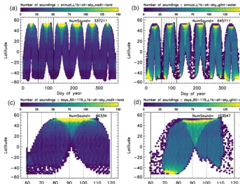
Figure 2a through 2d show the number of measurements as a function of latitude and day of year, with nadir–land (panels a and c) and glint–water (panels b and d) observations shown separately. The data are binned in increments of 1 d and 2◦ latitude. The values in these figures, and in the accompanying discussion, must be inflated by 240 to reflect expected real sounding densities at the full spatiotemporal resolution. Note that the figures in this section use L1b data collection density with no filtering. That is, no cloud–aerosol prescreening or post-L2FP filtering has been performed here, and these topics are discussed in later sections.
The most notable feature of the density data is the sinu-soidal pattern with a period of approximately 70 d, yield-ing'five repeat cycles per year. The nadir–land observa-tion density ranges from close to zero soundings per bin be-low∼30◦S latitude (where there is little land) to approxi-mately 25 soundings per bin (per day, per 2◦latitude) south-ward of∼20◦N latitude. Northward of∼20◦N latitude, the sampling density has significant dependences on latitude and time, with a maximum of more than 300 soundings per bin at the northern extremity (∼55◦N).
The pattern for glint–water viewing is qualitatively very similar, but with density 2 to 3 times higher than land across most of the subtropics. The data densities can be over 300 soundings per bin at high latitudes near the satellite orbit in-flection points. The simulated geometry used in this work takes into account the physical limitations of the PMA due to interference from the solar panels and other constraints on the ISS. These physical restrictions have an especially large impact on the Southern Hemisphere glint data, as seen around DOY 120, 180, and 240 in Fig. 2.
Figure 2e and d show the same data as a subset for the DOY range 60 to 119 (approximately March–April) to high-light the latitude and time dependence of the data collection across most of a single 70 d repeat cycle. Some interesting features, advantages, and limitations of these collection pat-terns are presented after the discussion of the seasonal maps that are shown next.
Figure 2.Simulated sounding densities for nadir–land(a, c)and glint–water(b, d)for the annual(a, b)and DOY 60–119(c, d)datasets. Data are binned in 1 d by 2◦latitude increments. Values should be inflated by 240 to reflect real expected sounding densities at the full spatial (eight footprints per frame) and temporal (3 Hz) acquisition rates. To account for the large dynamic range, the density scale has been truncated at 150, although the extreme high latitudes contain up to 300 soundings per bin in some cases.
under a million soundings total for the full year, with approx-imately 25 soundings in each 2◦bin over most of the globe per season. Presenting the data in this manner accentuates the high density of soundings at the orbit inflection points, al-though the drift in coverage with seasons is muted. The gaps in data collection so apparent in Fig. 2 are no longer observed when the data have been aggregated monthly or seasonally. This has implications for the spatial and temporal scales of science questions that can be probed with the OCO-3 obser-vations made from the ISS.
Figure 4 uses Hovmöller diagrams to illustrate some of the features of the sampling from the ISS precessing orbit. Panel (a) shows the observation latitude as a function of hours from local noon (HFLN) and day of year (DOY) for the full an-nual dataset. The dominance of the yellow shades suggests that a large fraction of the soundings are taken at latitudes greater than 50◦N. Panel (b) shows the HFLN as a function of latitude and DOY for the full annual dataset. Most of the observations are taken±5 h relative to local solar noon. Here the'70 d repeat cycle is evident, and the precession in ob-servation time as a function of latitude becomes clear.
Figure 4c and d show a subset of the data for DOY 60 to 119 (approximately March and April) to highlight some of the detail across a single repeat cycle. 10 d periods are de-noted with vertical lines in the diagrams. The data dropouts due to mechanical interference of the PMA by the ISS are
seen at the higher southern latitudes. In general, the diur-nal and spatial sampling pattern of OCO-3 aboard the ISS will vary significantly from the more familiar polar-orbiting satellites. This will have implications for the XCO2and SIF science questions that can be explored.
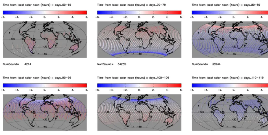
Figure 5 presents global maps of the sampling pattern for the six sets of 10 sequential days, highlighting both the spa-tial coverage and time-of-day sampling for a single repeat cycle. These maps clearly show the ascending–descending node variation in time, elucidating the drift in HFLN as a function of day for any given location. The interpretation of this complex sampling pattern by global flux inversion mod-els in an observing system simulation experiment (OSSE), as was performed for OCO-2 by Miller et al. (2007) and for GOSAT by Liu et al. (2014), is an interesting but unexamined issue that is outside of the scope of the current work.
3.2 Simulated instrument polarization angle and Stokes coefficients
polar-Figure 3.Seasonal L1b sounding density maps for 2◦latitude by 2◦longitude bins.(a)DJF,(b)MAM,(c)JJA, and(d)SON. Values should be inflated by 240 to reflect real expected sounding densities at the full spatial (eight footprints per frame) and temporal (3 Hz) acquisition rates.
Figure 5.Simulated OCO-3 sampling pattern for six 10 d periods, colored by the time in hours relative to local noon. The pixel size of individual footprints has been magnified for viewing purposes.
ized perpendicular to the long axis of the spectrometer slits.1 This is critical over strongly polarizing water surfaces but of lesser concern over land surfaces, which are only slightly po-larizing. Specifically, the vertically polarized component of light reflecting off a water surface is very low for incidence angles in a broad range about Brewster’s angle (53◦). If the instrument is oriented such that it only accepts the vertically polarized component for a given sounding then the measure-ment SNR is expected to be very low in clear-sky or nearly clear-sky scenes, making the retrieval of XCO2unreliable. The polarization angle of any particular sounding is a quan-tity that is calculable from the observing geometry and sen-sor orientation. The local meridian plane, formed by the lo-cal normal and the ray from the ground FOV to the satellite, forms the reference plane for polarization. The polarization angle of a measurement (φp) is then defined as the angle be-tween the axis of the instrument’s accepted polarization and this reference plane (Bösch et al., 2015). Since fundamental physics predicts that scattered light will be preferentially po-larized parallel to the plane of a horizontal surface, i.e., per-pendicular to the local meridian reference plane, the closer the OCO-3 polarization angle to 90◦(0◦), the more (less) re-flected sunlight incident on the instrument will pass through
1As noted in Crisp et al. (2017), the OCO-2 instrument was built
erroneously; it was intended to be sensitive only to light parallel to the long axis of the spectrometer slits. OCO-3 was built in the same manner. This error was mitigated on OCO-2 by yawing the space-craft in order to maximize the signal over ocean while simultane-ously maintaining sufficient electrical power generated from sun-light incident on the spacecraft solar panels. For OCO-3, electrical power comes from the ISS and is therefore a nonissue.
to the detectors, assuming a constant amount of polarization of the light.
The polarized intensity detected by OCO-2 or OCO-3 is given by
Imeas=mII+mQQ+mUU, (1)
whereIrepresents the total intensity, andQandUrepresent components of the linearly polarized portion of the light. The circular component of polarization,V, is ignored as it is typ-ically extremely close to zero in the atmosphere, and most instruments are designed to be insensitive to it. The so-called Stokes coefficientsmi for an instrument containing a polar-izer such as OCO-2 and OCO-3 are given by
mI= 1
2, (2)
mQ= 1
2·cos(2φp), (3)
mU =1
2·sin(2φp). (4)
Detailed optical modeling and laboratory tests were per-formed to simulate the effects of the PMA-induced changes to the polarization angle. The analysis shows that φp is largely driven by the PMA elevation angle with some in-fluence from the PMA azimuth angle. For elevation angles below 20◦, the polarization angle is nearly equal to the ele-vation angle of the PMA. In the nadir-observing mode, the sensitivity to polarization is essentially negligible. However, for all off-nadir measurements, i.e., glint, transition, target, and SAM modes, there will be a range of polarization angles as the elevation angle of the PMA is adjusted to view the ground target.
These effects are neatly summarized in Fig. 6, which shows contours of the theoretical O2A-band SNR as a func-tion of both solar zenith angle (SZA) and polarizafunc-tion an-gle for a specularly reflecting surface model (Cox and Munk, 1954) at a fixed wind speed of 8 m s−1. The constant polar-ization angle of OCO-2 at 30◦is designated by the horizon-tal dot-dashed line, while the polarization angle of OCO-3 assumed in this work is shown by the labeled dashed line, which used a simple but inexact parameterization of the re-lationship between the PMA elevation angle (ζPMA) and the polarization angle. In the figure, the actual range of polariza-tion angles for OCO-3 expected on-orbit using a more com-plete parameterization is indicated by the gray shaded area. As stated above, this range is closely tied to the PMA eleva-tion angle, which itself is closely related to the solar zenith angle at the glint spot. Note that actual on-orbit OCO-3 SNRs over ocean at the higher SZA values will be somewhat less than those depicted in Fig. 6 and Sect. 5, as OCO-3 will off-point from the true glint spot to avoid saturating its detectors, as was done for OCO-2 (Crisp et al., 2017).
3.3 Simulated meteorology, gas and cloud–aerosol fields
In our simulations, the vertical profiles of standard meteo-rological information needed to calculate realistic radiances were taken from the National Centers for Environmental Pre-diction (NCEP) (Saha et al., 2014). The NCEP database has a native spatial resolution of 2.5◦latitude by 2.5◦longitude (10 512 spatial points) with variables given on 17 vertical lay-ers every 6 h. For this work, the model was sampled at indi-vidual OCO-3 observations, defined by time, latitude, lon-gitude, and surface elevation for temperature, humidity, 2 m temperature, surface pressure, and winds. The data are inter-polated spatially and temporally to 26 vertical levels to create “scenes” for every individual OCO-3 sounding.
Vertical values of carbon dioxide for each sounding were sampled from the CarbonTracker 2015 database (CT2015) (Peters et al., 2007, with updates documented at http:// carbontracker.noaa.gov (last access: April 2019), which has a native spatial resolution of 2.0◦latitude by 3.0◦longitude (10 800 spatial points), with CO2 mole fractions given on 25 vertical layers every 3 h. Data are interpolated in space
Figure 6.Contour plot of the theoretical SNR versus solar zenith and polarization angles as determined from a Cox and Munk sur-face reflectance model. Results here are for the O2A band assuming
an 8 m s−1surface wind speed. Results for the CO2spectral bands and for other realistic wind speeds look qualitatively similar (not shown). The fixed OCO-2 operational polarization angle due to the 30◦instrument yaw is indicated by the horizontal dot-dashed line, while the simple relationship between the OCO-3 polarization an-gle and solar zenith anan-gle used in these simulations is indicated by the dashed line. The gray shaded region shows the range of the ex-pected on-orbit OCO-3 polarization angles determined from recent calculations.
and time to match individual OCO-3 soundings. Note that although the ISS ephemeris was taken from 2015, the CT database was sampled for 2012. Ultimately this makes no dif-ference to the overall outcomes reported in this paper (which are not focused on actual carbon cycle science), but it is im-portant to note that the simulations are representative of an Earth-like system, not the actual conditions on Earth at the time of the soundings.
3.4 Simulated land surface model and SIF
A model of the Earth’s surface is a critical component for the calculation of reflected solar radiances. For land sur-faces, scalar bidirectional reflectance distribution functions (BRDFs) were taken from the MODIS 16 dMCD43B1 prod-uct (Schaaf et al., 2002). For water surfaces, a fully polar-ized Cox and Munk model with a foam component based on wind speed was used. Additional details and citations can be found in the simulator Algorithm Theoretical Basis Doc-ument (ATBD) (O’Brien et al., 2009). Realistic estimates of solar-induced chlorophyll fluorescence from biological activ-ity were added to the O2A-band L1b radiances based on the implementation of Frankenberg et al. (2012). A static gross primary production (GPP) climatology of Beer et al. (2010), which is a mean monthly climatology based on the 18 In-ternational Geosphere–Biosphere Programme (IGBP) (Love-land and Belward, 1997) surface types at 0.5◦ by 0.5◦ lati-tude and longilati-tude resolution, is scaled to a daily average SIF value using the empirical scaling factor of Frankenberg et al. (2011). Daily average SIF is converted to instantaneous SIF via scaling by the instantaneous solar insolation relative to the average for that day and location. The wavelength depen-dence is a double Gaussian function as given in Frankenberg et al. (2012). Overall, this provides values of SIF that are rep-resentative in time (seasonal and diurnal cycle) and space (as a function of latitude and local plant physiology). It is worth noting that the use of the static GPP climatology does not al-low for interannual variability, but this has no effect on the single year of simulated data presented here.
3.5 Simulated L1b radiances
Radiances, as are expected to be observed by the OCO-3 instrument in space, are calculated using the same forward model (FM) that has previously been employed for GOSAT and OCO-2 simulation studies; e.g., O’Dell et al. (2012). The FM consists of an atmospheric model, surface model, instru-ment model, solar model, and radiative transfer model.
The solar spectrum is comprised of two parts: a pseudo-transmittance spectrum (Toon et al., 1999) and a solar con-tinuum spectrum (Thuillier et al., 2003) used to produce a high-resolution, absolutely calibrated input solar spectrum for the forward model (Bösch et al., 2015). For this work, the gas absorption coefficients, i.e., spectroscopy, of the OCO-2 operational B8 L2FP algorithm, ABSCO v5.0.0, were used. The instrument model, which includes the instrument line shapes (ILSs), radiometric characteristics, polarization sen-sitivity, and noise specifications, was taken from the OCO-3 thermal vacuum tests performed in September 2016. Noise was applied to the calculated radiances via the same model used for OCO-2, as described in Rosenberg et al. (2017). The radiative transfer calculation accounts for multiple scattering from clouds and aerosols as well as polarization, as described in O’Brien et al. (2009) and references therein.
4 Level 2 preprocessors and full physics retrieval algorithm
The primary data products for OCO-2 and OCO-3 are the column-averaged dry-air mole fraction of CO2(XCO2) and the solar-induced chlorophyll fluorescence, both of which can be used to help constrain the global carbon cycle; e.g., El-dering et al. (2017b) and Sun et al. (2017). For this work, the simulated L1b radiances were analyzed with the same tools used in OCO-2 operational data processing, as described in Sect. 4 of Eldering et al. (2017a). These steps include pre-screening, the level 2 full physics (L2FP) algorithm, qual-ity filtering, and the application of a bias correction (BC) for XCO2. This section briefly discusses each of the components as it relates specifically to the OCO-3 simulations. Relevant citations containing the full details are provided.
4.1 Preprocessors
Cloud screening was performed using only the A-band pre-processor (ABP), as described in Taylor et al. (2016). The ABP identifies cloud-contaminated soundings primarily via a threshold on the difference in retrieved and prior surface pressure in the oxygen A band, typically±25 hPa. Although operational OCO-2 data also utilize a weak filter on the ratio of CO2retrieved independently in the strong and weak CO2 bands by the IMAP–DOAS preprocessor (IDP), we did not implement this filter for cloud screening. The IDP CO2and H2O ratios were, however, used for post-L2FP retrieval qual-ity filtering and bias correction. In addition, IDP performs a retrieval of SIF, which is used as a prior for the full physics L2FP SIF retrieval that is included in the L2FP state vector as a necessary interferent parameter (see Sect. 3.5 of O’Dell et al., 2018). Both preprocessors neglect scattering in the at-mosphere (except Rayleigh scattering is included in ABP), making them computationally very efficient.
4.2 Full physics retrieval algorithm for XCO2
The soundings that were identified as clear by the ABP cloud flag were then run through the OCO-2 B8 operational L2FP retrieval algorithm. The algorithm was first described in Bösch et al. (2006) and Connor et al. (2008) prior to the failed launch of OCO-1 in February 2009, and it was later applied to GOSAT as described in O’Dell et al. (2012). Re-cent updates and a complete description of the modern B8 version of the algorithm can be found in Bösch et al. (2015) and O’Dell et al. (2018).
term. The high-spectral-resolution measurements of top-of-atmosphere reflected radiances measured by sensors such as GOSAT, OCO-2, or OCO-3 serve as the primary source of information in the retrieval. The measurements are coupled with an a priori state of the atmosphere (the state-vector ele-ments listed above) in order to constrain the inversion. Within the L2FP retrieval, modeled spectra are generated by a radia-tive transfer (RT) code as described in O’Dell et al. (2012) and Bösch et al. (2015). Although they share many compo-nents, the L2FP RT code base differs slightly from the RT model used to generate the simulated L1b radiances, thus creating a realistic error source in the simulation exercise. 4.3 Filtering and bias correction approach
The NASA operational procedure for both OCO-2 and GOSAT applies a quality filtering and bias correction (BC) process to the L2FP XCO2 (O’Dell et al., 2018). Correla-tions between variables and XCO2error variability are quan-tified and used to develop the filtering thresholds and lin-ear bias correction equations. The quality filtering is de-signed to remove soundings with anomalous XCO2 values relative to other soundings in close proximity, making use of the assumption that real variations in XCO2are quite small (<1 ppm) on small scales (<100 km). Some form of “truth” metric, or truth proxy, is required with which to calculate an “error” in XCO2. For operational OCO-2 data, several forms of a truth proxy are used, as detailed in Sect. 4.1 of O’Dell et al. (2018).
A similar treatment was applied to the OCO-3 simulation dataset. However, with simulations it was possible to use the actual true XCO2as the truth proxy in the QF and BC pro-cedures. There are both advantages and disadvantages to the circularity imposed by knowing the true values of the atmo-spheric state. In this case, we expect that the use of the truth data will result in an overly optimistic QF and BC. On the other hand, we do not have to consider errors in the truth proxy itself in our analysis, an issue of real concern when working with real measurements such as those from TCCON validation sites or model estimates of XCO2.
At its completion, the quality filtering and bias correc-tion procedure assigns to every sounding a binary flag in-dicating good (0) or bad (1) quality, as well as a BC value in units ppm. The operational OCO-2 BC equation contains three components: a correction based on retrieval variables (parametric), a correction for inter-footprint dependence, and a global bias, each calculated separately for land (combined nadir and glint) and ocean–glint. For the OCO-3 simulations the inter-footprint bias is not needed since only a single foot-print per frame was calculated. Explicit results from the pro-cedure as performed on the OCO-3 simulations are given in Sect. 5.3 and 5.4.
5 Results
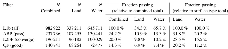
This section discusses characteristics of the L1b radiances, performance of the preprocessors, and application of the quality filtering and bias correction methodology before pre-senting the L2FP XCO2 results. In addition, we provide a brief analysis of the SIF determined by the IMAP–DOAS preprocessor retrieval. Table 1 summarizes the number of soundings in the simulated dataset at each stage of the analy-sis, broken down by nadir–land and glint–water observations. 5.1 Simulated L1b radiance characteristics
At a gross level, the characteristics of the simulated OCO-3 radiances are very similar to those from real OCO-2 mea-surements. The high-resolution spectra for OCO-3 (not shown) exhibit the expected absorption features that allow for cloud and aerosol screening and the retrieval of surface pressure and SIF (from the O2A band) and XCO2(from the weak and strong CO2bands).
However, some differences are expected between the two sensors in both measured signal and instrument noise due to the addition of the PMA and calibration characteristics of the spectrometers, e.g., dark noise, stray light, and ILS. Optical inefficiencies in the OCO-3 PMA will reduce the transmis-sion of light by about 17 % in the O2A band and 7 % and 5 % in the weak and strong CO2bands, respectively. To com-pensate for the effects of the PMA, the instrument aperture of the O2A band was increased. When all of the optical ele-ments and instrument changes are considered, the O2A band transmission of OCO-3 will be about 95 % of OCO-2, while the weak and strong CO2bands will have 75 % of the trans-mission of OCO-2, thus reducing the observed signal for the same scene.
The instrument calibration parameters for the OCO-3 sim-ulations reported here were derived from the September 2016 prelaunch thermal vacuum testing (TVAC), which was per-formed using an early version of the instrument telescope and without the PMA installed. The noise coefficients were ad-justed post hoc to account for the reduced optical throughput caused by the PMA, which was discussed in Sect. 2.2. Al-though the final thermal vacuum test of the OCO-3 payload, including the PMA, was completed in July 2018, analysis is still in progress to generate calibration coefficients from these data. Some values will remain fixed, while others will be regularly updated in-flight. Instrument performance will be reported in forthcoming papers postlaunch. Based on pre-liminary analysis, the updated instrument characteristics are not expected to change at a level that would greatly effect the results presented here.
radi-Table 1.Summary statistics of the filtering for each stage of the analysis. Results are shown for the nadir–land, glint–water, and combined soundings separately.
Filter N N N Fraction passing Fraction passing Combined Land Water (relative to combined total) (relative to surface type total)
Combined Land Water Land Water L1b (all) 982 922 337 211 645 711 100.0 % 34.3 % 65.7 % 100.0 % 100.0 % ABP (pass) 237 736 107 295 130 441 24.2 % 10.9 % 13.3 % 31.8 % 20.2 % L2FP (converge) 196 211 96 182 100 029 20.0 % 9.8 % 10.2 % 28.5 % 15.5 % QF (good) 140 741 68 264 72 477 14.3 % 6.9 % 7.4 % 20.2 % 11.2 %
ances using the 10 channels with the highest values, after fil-tering for outliers that occasionally exist due to cosmic rays or some other random electronic anomaly. The OCO noise model combines contributions from a constant background (dark noise) term and a photon (shot noise) term, the latter of which is proportional to the square root of the radiance (Rosenberg et al., 2017).
Figure 7 compares the OCO-2 SNR calculated from the operational noise model (solid traces) against OCO-3 (dashed traces) versus a measure of the surface brightness, parameterized as the albedo scaled by the cosine of the so-lar zenith angle:A·cos(SZA). Panel (a) displays the SNR of each spectral band for both sensors, while panel (b) shows the ratio of the two sensors’ SNR per spectral band. These data demonstrate that the only situation in which OCO-3 has a higher SNR than OCO-2 is in the O2 A band when A·cos(SZA)&0.15. This typically occurs over very bright deserts and during glint–water measurements when the sun is low in the sky. It is worth noting that the O2 A band is used primarily for cloud and aerosol detection and for the L2FP surface pressure retrieval as well as for SIF. In both the weak and strong CO2bands (green and red, respectively, in Fig. 7), OCO-3 always has a significantly lower SNR than OCO-2. This reduced SNR can be attributed to some combi-nation of increased noise in the instrument detectors and/or to a decreased signal incurred by the use of the PMA, a po-larizer in the telescope, and a larger center obscuration in the entrance optics.
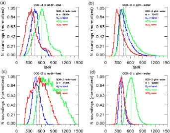
The overall SNR differences are captured in the his-tograms of Fig. 8, which compare the OCO-3 simulations with the real SNR for operational OCO-2 B8 measurements acquired in 2016. The operational OCO-2 data have been down-selected to include only a single footprint per frame and one sounding every 10 s to provide a fairer compari-son against the OCO-3 simulations. Both datasets have been screened using their respective L2FP quality flags, which were introduced in Sect. 4.3 and will be discussed in more detail in Sect. 5.3. At a gross level, the data look reasonably similar, although a few key distinctions stand out, particu-larly the fact that the slightly brighter OCO-3 O2A band is primarily due to a long tail of high values for glint–water soundings. The OCO-3 weak CO2band exhibits a
substan-tially lower SNR for glint–water compared to OCO-2, while the strong CO2band tends to be somewhat lower than OCO-2. These figures show that the OCO-3 data will include fewer data with SNR values over 600 and more data with SNR be-tween 200 and 400. Previous OCO-2 studies and experience with the real data show that an SNR of 200 is sufficient to achieve the desired precision of the retrieval algorithm. As will be shown in Sect. 5.5 and 5.6, the L2FP retrieval still provides good estimates of XCO2 and SIF on this set of OCO-3 simulated radiances, even with the lower SNR val-ues.
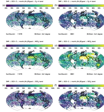
Maps comparing the simulated OCO-3 SNR to the opera-tional B8 OCO-2 data are shown in Fig. 9 for the month of April for each spectral band. Qualitatively, the overall pat-terns agree quite well, although the difference in latitudinal coverage from the two spacecraft is apparent as are differ-ences in the throughput, notably over the Amazon, the Sa-hara, and eastern China. A higher fraction of the soundings that converge in the L2FP retrieval are assigned a good qual-ity flag in the OCO-3 simulations (approximately 70 % ver-sus only about 40 % for real OCO-2 B8 data). The differences in throughput are likely driven by deficiencies in the simu-lation setup. In particular, there is a lack of a southern At-lantic anomaly model and a parameterized cloud and aerosol scheme in the L1b simulations with full realism. We expect that real on-orbit OCO-3 good quality sounding fractions will in reality be closer to the OCO-2 values, especially over the three continental areas mentioned above. For both sensors, the highest SNRs are obtained over unvegetated (bright) land and for glint–water when the sun is low in the sky, which produces a strong specular reflection. The lowest values of SNR occur when the sun is high in the sky and for vegetated (dark) land surfaces at higher latitudes. As with OCO-2, the weak CO2band displays the highest SNR values, while the O2A band and strong CO2bands have lower but comparable SNRs.
con-Figure 7.OCO-2 and OCO-3 mean SNR (averaged across footprints and channels) for each band as a function of the product of surface albedo and cosine of solar zenith angle(a). The quantity A cos(SZA)is proportional to the reflected sunlight off a surface. Panel(b)shows the ratio of OCO-3 SNR to OCO-2 SNR using a logarithmic abscissa scale. The small vertical lines represent A cos(SZA)for Railroad Valley at the winter solstice. OCO-3 SNR is lower at lower signal levels because it has a higher noise floor than OCO-2.
Figure 8.SNR histograms comparing simulated OCO-3(a, b)to operational B8 OCO-2(c, d)for nadir–land(a, c)and glint–water(b, d). The colors represent the three spectral bands, as described in the legend. Both datasets have been filtered using their respective L2FP quality flags. The median value for each spectral band is shown as a vertical dashed line in the corresponding color.
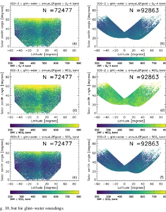
sequence of the ISS precessing orbit versus the polar orbit of OCO-2. It is also evident that the OCO-3 measurements span a much larger SZA range (∼75 to 0◦) compared to OCO-2. As was demonstrated previously in the histogram plots (Fig. 8), we find that for nadir–land the SNR values tend to be lower for OCO-3 compared to OCO-2 in all spec-tral bands, with the exception of a few high O2A-band SNRs around 20◦latitude that correspond to the Sahara. For glint– water soundings, there is a population of very high SNR
val-ues (>800) spanning the full latitudinal space at SZA∼60◦ due to the very bright specular glint spot achieved under these conditions.
lat-Figure 9.Maps comparing the SNR of OCO-3(a, c, e)to OCO-2(b, d, f)for each spectral band (rows) for the month of April binned in 2◦ latitude bins. Both datasets have been filtered using the L2FP quality flag. The operational OCO-2 data have been down-selected to include a single footprint and one sounding every 10 s to provide a fairer comparison against the OCO-3 simulations. The OCO-2 data also include both nadir and glint land soundings in addition to glint–water.
itude, we expect that the SNR distribution, which fundamen-tally drives the information content in the L2FP retrievals, will not be tied to latitude in the same way that it is for OCO-2. This has implications as to the spatial patterns of good quality XCO2and SIF retrievals, as will be discussed in the following sections.
5.2 Preprocessor performance
For this simulation experiment only the ABP cloud flag was used to select soundings, although real operational sound-ing selection is expected to be slightly more elaborate (see Sect. 2 of O’Dell et al., 2018). In particular, no IDP variables were used in the L2FP sounding selection here, although they were used later in the post-filtering and bias correction. The results shown in Table 1 indicate that about a quarter (24.2 %) of all of the observations passed the ABP cloud flag, leaving
about 250 000 to run through the L2FP retrieval. By viewing mode, approximately one-third (31.8 %) of the nadir–land and one-fifth (20.2 %) of the glint–water observations passed the ABP cloud flag. These statistics are roughly similar to those seen in real OCO-2 operational processing.
Figure 12 shows maps of the clear-sky fractions in each 2◦spatial bin (left) and the resulting clear-sky sounding den-sities (right). As expected, the highest fraction (up to about 75 %) of the scenes pass in the arid land regions, where there are few clouds and aerosols. The southern subtropical oceans also tend to have areas of moderately high passing rates of
Figure 10.Comparison of the nadir–land SNR of OCO-3(a, c, e)to OCO-2(b, d, f)for each spectral band (rows) for the full annual dataset. Both datasets have been filtered using the L2FP quality flag. The operational OCO-2 data have been down-selected to include a single footprint and one sounding every 10 s to provide a fairer comparison against the OCO-3 simulations.
are qualitatively very similar to those seen in Fig. 1 of O’Dell et al. (2018) for OCO-2 operational B8 data.
Figure 12b confirms that the highest density of cloud-free soundings (more than 100 per 2◦bin) is found over the arid regions of the globe, as expected. In addition, a large num-ber of soundings are found over Northern Hemisphere land at the satellite orbit inflection points. Much of the temperate land regions contain∼30–50 soundings per bin, while few soundings remain over tropical forests. In glint–water view-ing, the regions of high clear-sky fraction have ∼50 to 80 soundings per 2◦ bin, while the cloudy areas contain only ∼10 soundings per bin selected for processing by the L2FP retrieval. Recall that on-orbit OCO-3 sounding densities will be approximately 240 times greater due to the reduced spa-tiotemporal sampling used in this simulation set.
5.3 Application of XCO2quality filtering
The L2FP retrieval algorithm described in Sect. 4.2 was ap-plied to the cloud-screened set of soundings, and then, as with operational OCO-2 data, a set of post-processing filters were implemented to determine the binary XCO2quality flag (QF) for each sounding. Details of the methodology are doc-umented in O’Dell et al. (2018). Here, the true XCO2 for each sounding was used as the truth metric to assess residual biases and errors. This provides perhaps an overly optimistic interpretation of the results and should be considered an up-per limit on the actual up-performance expected from on-orbit OCO-3 measurements.
Figure 11.Same as Fig. 10, but for glint–water soundings.
methodology was applied independently to the nadir–land and glint–water scenes, as is done with operational OCO-2 data. A total of 11 variables were used to form the QF for nadir–land, while 9 were used for glint–water. Not surpris-ingly, many of the same variables are selected for quality fil-tering the OCO-3 simulations as were used in the operational OCO-2 procedure (see, e.g., Figs. 10 and 11 of O’Dell et al., 2018). Approximately 70 % of the soundings that converged in L2FP were assigned a good QF.
The quality filtering process had similar impacts on data volume across all months (not shown). On average, global data densities of good QF soundings in the simulations were 11 000 to 12 000 soundings per month or 33 000 to 36 000 per season. When using the full spatiotemporal resolution, this translates to approximately 2.5 million soundings per month (7.5 million per season), similar to the density of OCO-2 B8 data.
Figure 13 shows seasonal plots of the fraction (left col-umn) and number (right colcol-umn) of soundings assigned a good QF for each season (DJF, MAM, JJA, SON) binned in 4◦degree latitude–longitude bins. The spatial patterns are useful, but the absolute numbers need to be inflated by 240 to reflect actual predicted on-orbit throughput.
In general, the QF throughputs for glint–water are quite high (>70 %) in the tropics and subtropics (<30◦latitude) and display little seasonal cycle. The QF throughput is per-sistently low for glint–water observations at the turnaround latitude in the winter hemisphere. The QF throughputs are more varied for nadir–land observations, and a modest sea-sonal cycle is seen for some regions. But overall, the results look qualitatively similar to those from OCO-2 for the B8 operational dataset and demonstrate that the methodology is a robust procedure.
5.4 Bias correction of XCO2
The final bias correction (BC) for the OCO-3 simulations in-corporates four of the QF variables for nadir–land and three for glint–water as shown in Table 4. Figure 14 illustrates how the final BC parameters for land affect the XCO2error. Each panel shows median binned values of the XCO2 error (re-trieved minus true in ppm) versus a particular retrieval vari-able (heavy, black dots). Also shown are the range in XCO2 error (thin vertical bars) and the least-squares linear fit (thin dashed line). To provide context, the relative histogram of points is shown in the background by the shaded gray region. The slope of the fit, the standard deviation of the XCO2error post-BC, and the percent of the variance explained by this variable are given in the legend. The original standard devia-tion is shown in the upper left panel for reference.
For land, 25 % of the variance is explained by the differ-ence in the L2FP-retrieved surface pressure from the prior (denoted dp), while another 15 % is explained by the square root of the combined retrieved aerosol optical depth (AOD) from dust, water cloud, and sea salt (DWS). An additional
3 % and 2 % are explained by the L2FP fine-mode AOD and the water vapor scaling factor, respectively. We believe that a minor indexing bug found in the simulated meteorology is re-sponsible for the reliance on water vapor. The final reduction in XCO2error is shown in Table 5, which gives the standard deviations (σ) in the retrieved XCO2with and without QF and BC. For land,σwas reduced from 1.88 to 0.85 ppm after application of both QF and BC.
Figure 15 is similar to Fig. 14, but for the glint–water scenes. Here, 18 % of the variance in XCO2error is explained by the IDP CO2ratio, while another 16 % is explained by the ABP dP. An additional 7 % is explained by the L2FP dP. The need for two preprocessor variables in the glint–water bias correction hints that the prescreening for clouds may not have been stringent enough. Use of the IDP results for prescreen-ing on real OCO-3 data may alter this outcome. As seen in Table 5, the XCO2σ was reduced from 2.15 to 0.52 ppm for glint–water soundings after application of both QF and BC. It is likely that the smaller QF–BCσfor glint–water (0.52 ppm) relative to nadir–land (0.85 ppm) is driven by L2FP retrieval interference errors such as albedo and aerosols, which vary more over land, as concluded by Worden et al. (2017) in their study of OCO-2 B7 data.
There are notable similarities and differences in the se-lected variables when comparing between the OCO-3 sim-ulations and either real OCO-2 data (Sect. 4.3.1 of O’Dell et al., 2018) or OCO-2 simulations (Kulawik et al., 2018). In all cases the L2FP dp is found to be the primary bias cor-rection parameter for land and water soundings. Both the real OCO-2 data and the simulated OCO-3 land data rely on a form of the aerosol parameterization for bias correction (DWS for the former and DWS and fine-mode aerosols for the latter). This stands to reason as aerosols are highly vari-able over land and have been shown to be a strong source of interference error (Connor et al., 2016).
A key difference is that the L2FP variable CO2grad del (δ∇CO
2), a measure of the change in the retrieved vertical
profile of CO2relative to the prior (see Eq. 5 in O’Dell et al., 2018), does not show up as a strong bias correction parame-ter in the simulated OCO-3 dataset. Kulawik et al. (2018) dis-cuss in detail the ties betweenδ∇CO
2, the L2FP prior CO2,
and the partitioning of CO2 in the upper and lower atmo-sphere in the retrieved state vector. At this time we have no real explanation as to why δ∇CO
2 is not showing up as a
bias correction term in the OCO-3 simulations. Analysis of on-orbit OCO-3 data, when available, will be revealing as to whether this is due to some fundamental difference in the OCO-3 measurements or perhaps associated with something particular in the retrieval setup.
Table 2.Variables and thresholds used for quality filtering in the OCO-3 simulations for nadir–land. The cumulative fraction of passing scenes is also given. Note that the need for the water vapor scale factor (L2FP WV scale) is likely due to a recently discovered bug in the simulator code that introduced a mismatch between the vertical profile in the scene and meteorology files.
Variable short name Variable description QF range Cum. frac. pass
IDP CO2ratio ratio of the CO2value retrieved in the 1.61 and 2.0 µm bands from the IDP [0.9, 1.03] 88.7 %
IDP H2O ratio ratio of the H2O value retrieved in the 1.61 and 2.0 µm bands from the IDP [0.88, 1.1] 85.6 %
L2FP dp difference between the retrieved and prior surface pressure from the L2FP retrieval [−6.0, 7.0] 81.6 %
L2FP total AOD combined optical depth from all aerosol and cloud species from the L2FP retrieval [0.0, 0.4] 79.1 %
L2FP water AOD optical depth of water cloud from the L2FP retrieval [0.0008, 0.1] 77.3 %
L2FP fine-mode AOD combined optical depth of fine-mode aerosol particles from the L2FP retrieval [0.0, 0.08] 74.8 %
L2FP WV scale water vapor profile scaling factor from the L2FP retrieval [0.84, 0.95] 73.7 %
ABP dp difference between the retrieved and prior surface pressure from the ABP retrieval [−25.0, 4.0] 71.7 %
L2FPδ∇CO
2 a measure of the change in the CO2profile shape versus the prior [−40.0, 40.0] 71.2 %
from the L2FP retrieval (in plain text denoted co2_grad_del)
L2FPχ2O2A the chi-squared goodness-of-fit statistic from the L2FP retrieval [0, 1.25] 71.1 %
L1b signal 3/1 ratio of the 2.0 to 0.76 µm spectral band from the measured L1b radiances [0.075, 0.4] 70.7 %
Table 3.Same as Table 2, but for glint–water soundings.
Variable short name Variable description QF range Cum. frac. pass L2FP WCO2albedo slope albedo slope term of the 1.61 µm spectral band [0.1, 100.0] 84.3 %
from the L2FP retrieval
ABP dp difference between the retrieved and prior surface pressure [−50.0,−3.0] 81.7 % from the ABP retrieval
L2FP dp difference between the retrieved and prior surface pressure [−5.0, 2.0] 75.0 % from the L2FP retrieval
IDP CO2ratio ratio of the CO2value retrieved in the 1.61 and 2.0 µm bands [1.0005, 1.015] 73.5 %
from the IDP retrieval
IDP H2O ratio ratio of the H2O value retrieved in the 1.61 and 2.0 µm bands [0.88, 1.03] 72.6 %
from the IDP retrieval L2FPδ∇CO
2 a measure of the change in the CO2profile shape versus the prior [−30.0, 60.0] 72.4 %
from the L2FP retrieval (in plain text denoted co2_grad_del)
L2FP total AOD combined optical depth from all aerosol and cloud species [0.0, 0.25] 72.2 % from the L2FP retrieval
Solar zenith angle solar zenith angle at the local target [0.0, 63.0] 70.4 % contained in the geolocation
with respect to spectroscopic lookup tables and meteorol-ogy. These results underscore the conclusion that even given nearly perfect alignment of the retrieval model with the truth, there are still retrieval errors that induce biases and scatter into the estimates of XCO2as explored in detail in Kulawik et al. (2018). This is particularly true of aerosols, which are a continued known source of trouble in virtually all retrievals of greenhouse gases from space (Aben et al., 2007; Butz et al., 2009; Nelson and O’Dell, 2019).
5.5 Retrieved XCO2characteristics after filtering and
bias correction
One of the objectives of this study was to analyze the er-ror on the retrieved XCO2 from OCO-3. Here the “actual” error is given as the retrieved value minus the known truth (after applying the averaging kernel correction) and is
de-noted 1XCO2. The “predicted” error is an L2FP retrieval state-vector parameter that provides the theoretical error due to the combination of measurement noise plus smoothing and interference errors, as discussed in Bösch et al. (2015). The actual errors in the simulated framework are expected to be lower than those seen in OCO-2 operational data, while the predicted errors should be roughly equivalent due to use of a similar instrument model and retrieval algorithm.
sig-Figure 13.Maps of the seasonal throughput(a, c, e, g)and the resulting sounding densities(b, d, f, h)in 4◦latitude–longitude bins for soundings assigned a good QF. Inflate densities by 240 to account for on-orbit spatiotemporal sampling.
nificant population of glint–water soundings with large neg-ative biases up to about−12 ppm.
The seasonal spatial distributions of 1XCO2 are shown in the maps in Fig. 18. These can be compared to Fig. 19 of O’Dell et al. (2018). While the qualitative patterns of ac-tual XCO2errors are quite different between OCO-2 B8 and simulated OCO-3 data, note that the dynamic range of the scale is much lower for OCO-3 (±1 ppm) compared to
Table 4.Bias correction parameters for the OCO-3 simulation. Only the prior (dp) terms have units (hPa), while the other parameters are unitless. Again, the need for a water vapor scaling factor bias correction term is likely due to an indexing bug in the L1b simulator code. The “DS” AOD is the combined optical depth of dust and sea salt aerosols.
Nadir–land Glint–water global bias is 0.18 global bias is 0.0 Variable short name Variable description BC slope, offset BC slope, offset L2FP dp difference between the retrieved and prior surface pressure −0.20, 1.0 (hPa) −0.21, 0.0 (hPa)
from the L2FP retrieval
L2FP WV scale water vapor profile scaling factor from the L2FP retrieval 14.0, 0.9 n/a L2FP
√
DWS AOD combined optical depth from the dust, water, and sea salt −7.6, 0.0 n/a aerosol species from the L2FP retrieval
L2FP fine-mode AOD combined optical depth of fine-mode aerosol particles from 14.0, 0.0 n/a IDP CO2ratio the L2FP retrieval ratio of the CO2value retrieved in the 1.61 n/a −170.0, 1.003
and 2.0 µm bands from the IDP retrieval
ABP dp difference between the retrieved and prior surface pressure n/a −0.053, 0.0 [hPa] from the ABP retrieval
n/a: not applicable.
Figure 14. Final bias correction variables used for nadir–land scenes illustrating the correlation of the actual error (1XCO2
de-fined as retrieved – true) as a function of variable value. The leading retrieval parameters that explain the maximum variance for land are the L2FP prior (dp), L2FP H2O scale factor, and two L2FP aerosol terms. The original standard deviation (σ) of the dataset is given in the upper part of the first panel, with the cumulative reduction inσ
and percent variance explained given in the lower right.
Table 5.Comparison of the standard deviation (σ) in XCO2before
and after QF and BC.
Land–nadir Ocean–glint
N 96 182 100 029
σ raw 1.88 ppm 2.15 ppm
σ BC 1.79 ppm 1.76 ppm
σraw QF 1.14 ppm 0.67 ppm
σQF, BC 0.85 ppm 0.52 ppm
For the OCO-3 simulations, after QF and BC have been applied, the errors are largely uncorrelated with any geophys-ical or retrieval parameters. Specifgeophys-ically, we used the glint– water soundings to check for correlation of both the raw and BC XCO2data against latitude, solar zenith angle, polariza-tion angle, SNR (per spectral band), and the true aerosol opti-cal depth. The results are summarized in Table 6. It is worth noting that the true AOD was not used as a bias fitting pa-rameter, yet there is a high reduction in the correlation with 1XCO2. The very small slopes, offsets, and linear correla-tion coefficients that remain after applicacorrela-tion of the QF–BC indicate that remaining errors in the XCO2are likely driven by retrieval errors such as the aerosol parameterization (Nel-son et al., 2016b).