ISSN 2291-8639
Volume 15, Number 1 (2017), 75-85 http://www.etamaths.com
OPTIMALITY AND DUALITY DEFINED BY THE CONCEPT OF TEMPERED FRACTIONAL UNIVEX FUNCTIONS IN MULTI-OBJECTIVE OPTIMIZATION
RABHA W. IBRAHIM
Abstract. In this paper, we purpose the concept of tempered Univex functions by utilizing a tem-pered fractional difference-differential operator type Caputo. This instruction indicates a new class of these functions in some optimal problems by exemplifying the settings on the modified formula. We call it the class of tempered fractional Univex functions. Our study is based on the strong, weak, converse, and strict converse duality propositions. A Multi-objective optimal problem includes the new process is disentangled.
1. Introduction
In 1989, Dunkl imposed a difference-differential operator [1] setting on some Euclidean space and realizing the commutative law for a differentiable function on Rn. This operator can be employed in various parts in pure mathematics, such as Lee algebra, Clifford algebra and complex analysis. In 1998, Rosler and Voit acquired into consideration this operator to adapt the tool of the Markov Processes [2]. Unevenly, these operators can be expected as a simplification of the partial derivatives and various constructions of operators like the Laplace operator, the Fourier transform, and the Hermite polynomials. Also, these operators convoluted in famous processes such as the Brownian motion and the Cauchy processes.
Recently, this operator and its some simplifications have improved significant care in many fields of mathematics and physics. They shield a helpful method in the study of special functions and they are closely related with definite demonstrations of degenerate affine Hecke algebras. Furthermore, Dunkl operator is obviously convoluted in the algebraic explanation of definite devotedly resolvable quantum multi-body systems. It can be used to identify the generalized method of the heat equation, which is called the Dunkl heat equation. It can be recommended to adapt the idea of moments of probability measures onRn. Our goal is to generalize the Dunkl operator in view of the tempered fractional calculus and propose it to simplify the class of non-linear Univex functions. This class typically appears in many non-linear multi-objective problems. The benefit of exploiting the Dunkle operator is that this operator deals with multi-dimensional spaces. Moreover, the author extend it to the complex plane and provided a modified differential-difference Dunkl operator in the open unit disk. The study was in the field of geometric function theory [3].
Fractional calculus is the most important branch of mathematical analysis, because it refers to the non-linearity studies in all science. The most famous operators are the Riemann-Liouville, Caputo (continuous operators) and Grunwald-Letnikov (discrete operator) (see [4], [5]). It has been presented the fractional calculus discoveries usage in many categories of science and engineering, containing fluid flow, diffusive transport theory, electrical networks, electromagnetic theory, probability and statistics. The tempered fractional diffusion idea was established in statistics. This idea has demonstrated useful applications in geophysics and finance [6]. Moreover, it applied to introduce a fractional multi-objective function in optimal control [7].
Received 15th May, 2017; accepted 28thJuly, 2017; published 1stSeptember, 2017.
2010Mathematics Subject Classification. 34A08, 26A33, 49J35.
Key words and phrases. fractional calculus; fractional differential operator; fractional differential equation; univex function.
c
2017 Authors retain the copyrights of their papers, and all open access articles are distributed under the terms of the Creative Commons Attribution License.
In this study, we aim to generalize the concept of tempered Univex functions by utilizing a tempered fractional differential-difference operator (Dunkl operator), based on different types of fractional cal-culus. This study gives us a new class of these functions in some optimal problems by illustrating conditions on the generalized functions. We call it the class of tempered fractional Univex functions. The strong, weak, converse, and strict converse duality theorems are proposed. The main tool employed in the analysis is based on the tempered Caputo operator.
2. Handling
We need the following concepts in the sequel of the article:
2.1. Dunkl operator. Suppose the two column vectors x = (x1, ..., xn) and v = (v1, ..., vn) ∈ Rn with their dot productx.v=xT.v=Pn
i=1vixi.The operator through the hyper-plane is defined by
σvx =x−2
v.x v.vv. In a matrix form, we have
σv = I−2
vvT vTv.
Note thatσv can be represented by a symmetric matrix. The Dunkl operator is formulated by:
Diφ(x) =
∂ ∂xi
φ(x) + X
v∈R+
kv
(1−σv)φ(x)
v.x vi, i= 1, ..., n,
whereviis the i-th component ofv,1≤i≤n, x∈ Rn., andφsmooth function onRn.Whenkv= 0,
then we have
Diφ(x) =
∂ ∂xi
φ(x).
One of the outcomes of these operators is satisfying
Di(Djφ(x)) =Dj(Diφ(x)). (2.1)
Moreover, the operator achieves the product
Di[φ(x)ψ(x)] =ψ(x)Diφ(x) +φ(x)Diψ(x).
Note that, ifφ is a polynomial of degree n, then (1−σv)φ(x)/v.x is a polynomial of degree n−1.
Moreover, the path of the Dunkl process onto a subset ofRn is collected by the set S={x∈Rn: x.v >0, ∀v∈R+}.
Finally, Dunkl processes are formulated as the Markov processes which achieve the Dunkl heat equation
∂ ∂t−
1 2
n X
i=1
D2i = 0.
2.2. Fractional calculus. The Cauchy formula for frequent integration, to be specific as follows:
(Inφ)(χ) = 1 (n−1)!
Z χ
0
(χ−t)n−1φ(t)dt,
drives in an explicit way to a generalization for realn. Utilizing the gamma function to take off the discrete nature of the factorial function allows us a natural candidate for fractional usage of the integral operator.
(Iαφ)(χ) = 1 Γ(α)
Z χ
0
(χ−t)α−1φ(t)dt
This operator is well-defined and it is represented to the classical fractional calculus, which is called the Riemann-Liouville fractional integral operator. It is straightforward to show that the integral operator achieves the semi-group property of fractional differ-integral operators
(Iα)(Iβφ)(χ) = (Iβ)(Iαφ)(χ) = (Iα+βφ)(χ) = 1 Γ(α+β)
Z χ
0
Corresponding to the above fractional integral operator and for a general functionφ(χ) and 0< α <1, the complete fractional derivative is defined as follows:
Dαφ(χ) = 1 Γ(1−α)
d dχ
Z χ
0
φ(t) (χ−t)αdt.
For the fractional power α < 1, since the gamma function is sloppy for values whose real part is a negative integer with the imaginary part is equal to zero, it is important to employ the fractional derivative after the integer derivative has been accurate. For example,
D5/4φ(χ) =D1/4D1φ(χ)=D1/4 d dχφ(χ)
.
In general, calculatingn-th order derivative over the integral of order (n−α),is given by the formula
aDαχφ(χ) =
dn
dχn aD
−(n−α) χ φ(χ) =
dn
dχn aI n−α χ φ(χ).
The Riemann-Liouville calculus admits a fast converge, historical property, natural generalization and wide applications in almost all science. One of the most property of this calculus is as follows:
Dαχm= Γ(m+ 1) Γ(m−α+ 1)χ
m−α, m
≥0.
There is another fractional differential operator called the Caputo operator, which is defined as follows:
C aD
α χφ(χ) =
1 Γ(n−α)
Z χ
a
φ(n)(τ)dτ (χ−τ)α+1−n.
This type of fractional differential operator is applied to find the solutions of fractional differential equations with initial conditions.
2.2.1. Tempered fractional calculus. The Riemann-Liouville tempered fractional derivative is formed as follows [9]
ˆ
Dα,λφ(χ) =e−λχDα eλχφ(χ)
−λαφ(χ), λ≥0. And the The Caputo tempered fractional derivative is formed as follows
C aDˆ
α,λφ(χ) = ˆDα,λ[φ(χ)− n−1 X
i=0
χi
i!φ
(i)(0)], λ≥0,
whereφ(i) is the derivative of orderi, andnis the upper integer value less thanα.Whenλ= 0, the
above equation reduces to the usual formula of the Caputo operator.
2.3. Tempered-Dunkl operator. Based on the Caputo tempered fractional calculus, assume that the fractional partial derivative is denoted byCaDˆα,λ.Then forx∈Rnwe receive the tempered Dunkl
operator as follows:
Dα,λi φ(x) =CaDˆ α,λ i φ(x) +
n X
i=1, v∈R+
kv
(1−σv)αφ(x)
v.x vi, (2.2)
i= 1, ..., n, 0< α <1,
where C aDˆ
α,λ
i is denoted the fractional derivative with respect the component xi, R+ is a positive
subsystem, satisfying for allu∈R+, u.v >0.Dunkl operators in the direction ofy∈Rn is defined as follows:
Dα,λφ(x) =
n X
i=1
yiDα,λi φ(x).
Proposition 2.1Letφ(x) be analytic function converging in the interval (0, ρ] with the approximate form
φ(x) =
∞
X
m=0
amxm+λ, λ >−1.
Then
Dα,λi Dβ,λj φ(x)=Djβ,λDα,λi φ(x), α, β∈(0,1), i= 1, ..., n.
Proof. In view of Theorem 3 in [3] and (2.1) , we have
Dα,λi Dβ,λj φ(x)= Dα,λi ∂
β
∂xβjφ(x) +
X
v∈R+
kv
(1−σv)βφ(x)
v.x vj
= Dβ,λj ∂
α
∂xα i
φ(x) + X
v∈R+
kv
(1−σv)αφ(x)
v.x vi
=Dβ,λj Dα,λi φ(x).
Proposition 2.2Letφandψbe power functions inx.Then
Dαi[φ(x)ψ(x)] =ψ(x)Dαiφ(x) +φ(x)Dαiψ(x).
Proof. By applying the fractional generalization of the Leibniz rule of the Caputo derivative [8]
∂α
∂xα[φ(x)ψ(x)] =
∞
X
k=0
Γ(α+ 1)
Γ(α−k+ 1)Γ(k+ 1)∂
α−kφ(x)∂kψ(x),
we conclude the desire result.
2.4. Tempered Univex function. In this subsection, we generalize the concept of tempered Univex function, by using the fractional calculus. Let Ω be a nonempty subset ofRn, η: Ω×Ω→Rm, ξ be an arbitrary point of Ω andh: Ω→Rm, φ:Rm→R.
Definition 2.1A differential function his said to be a tempered fractional univex function of order α∈(0,1) in the direction ofξ∈Ω if for allx∈Ω,we have
η(x, ξ).Dα,λh(x)≤φh(x)−h(ξ),
where
Dα,λh(x) =
n X
i=1
ξiDα,λi h(x), ξ= (ξ1, ..., ξn).
The advantage of using the tempered fractional Dunkl operator, is that can be acted on multi-dimensional Euclidean spaces as well as it can be defined a parametric family of deformations of the polynomial . Therefor, it can be employed in non-linear multi-objective problem
M inimize Ψ(x) = ψ1(x), ..., ψm(x)
subject to Θ(x)≤0, (2.3)
where Ψ : Ω→Rmand Θ : Ω→Rpand 0 is the zero vector inRp.The function Ψ(x) can be applied in various studies. It can be considered as a utility function over some set of needs (goods), cost function of production presented a fixed quantity produced, growth function and others.
Definition 2.2 A point ξ ∈Λ := {x∈ Ω : Θ(x)≤ 0} is said to be an efficient solution of (2.3), if there exists nox∈Λ,such that Ψ(x)≤Ψ(ξ).And it is called a weak efficient solution if Ψ(x)<Ψ(ξ).
Definition 2.3 The couple (Ψ,Θ) is called (α, λ, ρ, η, ϑ)-type univex at ξ∈ Ω if for all x∈Λ such that
η1(x, ξ).Dα,λΨ(x) +ρ1kϑ(x, ξ)k2≤φ1
Ψ(x)−Ψ(ξ)
and
η2(x, ξ).Dα,λΘ(x) +ρ2kϑ(x, ξ)k2≤ −φ2
Θ(x)−Θ(ξ),
whereη1: Ω×Ω→Rm, η2: Ω×Ω→Rp, ϑ: Ω×Λ→R, φ1:Rm→R, φ2:Rp→Randρ1, ρ2∈R. We have the following facts:
Remark 2.1
• If φ1
Ψ(x)−Ψ(ξ) ≤ 0 ⇒ η1(x, ξ).Dα,λΨ(x) ≤ −ρ1kϑ(x, ξ)k2 and φ2
Ψ(x)−Ψ(ξ) ≥
0⇒η2(x, ξ).Dα,λΨ(x)≤ −ρ2kϑ(x, ξ)k2.Then the couple (Ψ,Θ) is called weak pseudo-quasi
(α, λ, ρ, η, ϑ)-type univex atξ∈Ω.
• If φ1
Ψ(x)−Ψ(ξ) ≤ 0 ⇒ η1(x, ξ).Dα,λΨ(x) < −ρ1kϑ(x, ξ)k2 and φ2
Ψ(x)−Ψ(ξ) ≥
0⇒η2(x, ξ).Dα,λΨ(x)<−ρ2kϑ(x, ξ)k2.Then the couple (Ψ,Θ) is called strong pseudo-quasi
(α, λ, ρ, η, ϑ)-type univex atξ∈Ω.
3. Results
In this section, we investigate some sufficient optimality conditions for a point to be an efficient solution of (2.3) under the tempered (α, λ, ρ, η, ϑ)-type Univex.
Theorem 3.1. Let ξbe an initial solution of the multi-objective problem (2.3) andc1 andc2 be two non-negative constants such that
(A) Θ(ξ) = 0;
(B) c1 η1(x, ξ).Dα,λΨ(x)+c2 η2(x, ξ).Dα,λΘ(x)≥0;
(C) The couple (Ψ,Θ) is a strong (or weak ) pseudo-quasi(α, λ, ρ, η, ϑ)-type univex at ξ∈Ω; (D) u≤0∈Rm⇒φ
1(u)≤0 andv≥0∈Rp⇒φ2(v)≥0; (E) c1ρ1+c2ρ2≥0.
Thenξis an efficient solution of (2.3).
Proof. Suppose that ξis not an efficient solution of (2.3), then there existsx∈Λ such that Ψ(x)≤ Ψ(ξ).By the assumptions (A) and (D), we have
φ1(Ψ(x)−Ψ(ξ))≤0, and φ2(Θ(ξ))≥0. (3.1)
In view of the assumption (C), we get
c1 η1(x, ξ).Dα,λΨ(x)<−c1ρ1kϑ(x, ξ)k2 (3.2)
and
c2 η2(x, ξ).Dα,λΘ(x)≤ −c2ρ2kϑ(x, ξ)k2. (3.3)
Summing the above inequalities and utilizing (E), we conclude that
c1 η1(x, ξ).Dα,λΨ(x)
+c2 η2(x, ξ).Dα,λΘ(x)
<− c1ρ1+c2ρ2
kϑ(x, ξ)k2
≤0,
which contradicts the assumption (B). Hence,ξ is an efficient solution of (2.3). This completes the proof.
Theorem 3.2. If the following conditions are satisfied:
(A) ξis a weakly efficient solution of (2.3); (B) Θis continuous inξ;
Then there are two constantsc1≥0 andc2≥0 such that
c1 η1(x, ξ).Dα,λΨ(x)
+c2 η2(x, ξ).Dα,λΘ(x)
≥0,
x∈Ω, c2Θ(ξ) = 0, η1: Ω×Ω→Rm, η2: Ω×Ω→Rp
.
Proof. Our aim is to show that the system
η1(x, ξ).Dα,λΨ(x)<0, η2(x, ξ).Dα,λΘ(x)<0,
has no solution forx∈Ω.Let the system has a solutiony∈Ω.By the assumption (A), we have
Ψ(ξ+1y)<Ψ(ξ) and Θ(ξ+2y)<Θ(ξ),
for sufficient small arbitrary constants 1, 2 > 0. Now, we let ¯x := ξ+2y; which implies that
¯
x∈Λ∩N2(ξ) thus by (B) and (C), we have Θ(ξ+2y) = Θ(¯x)<0; which contradicts (A), whereξ
is a weak solution. Therefore, the above inequalities are non-negative. Hence, in view of (C) these are two constantsc1 andc2satisfy the inequality
c1 η1(x, ξ).Dα,λΨ(x)
+c2 η2(x, ξ).Dα,λΘ(x)
≥0,
with the propertyc2Θ(ξ) = 0. This completes the proof.
Next, we consider the dual problem of (2.3) as follows:
M ax Ψ(χ) = ψ1(χ), ..., ψm(χ)
subject to c1 η1(x, χ).Dα,λΨ(x)+c2 η2(x, χ).Dα,λΘ(x)≥0,
c2Θ(χ)≥0,
(3.4)
whereχ∈Ω, c1and c2 be two non negative constants.
Theorem 3.3. Letx, χbe initial solutions of the multi-objective problems (2.3)and (3.4)respectively. If
(A) The couple (Ψ,Θ) is a strong (or weak ) pseudo-quasi(α, λ, ρ, η, ϑ)-type univex at ξ∈Ω; (B) u≤0∈Rm⇒φ1(u)≤0 andv≥0∈Rp⇒φ2(v)≥0;
(C) c1ρ1+ρ2≥0; thenΨ(x)Ψ(χ).
Proof. Suppose that Ψ(x)≤Ψ(χ). Sincec1ρ1+ρ2≥0 then by (B), we obtain
φ1(Ψ(x)−Ψ(χ))≤0
φ2(Θ(χ))≥0.
In virtue of the assumption (A) the above inequalities yield
η1(x, χ).Dα,λΨ(χ)
<−ρ1kϑ(x, χ)k2
η2(x, χ).Dα,λΘ(χ)≤ −ρ2kϑ(x, χ)k2,
consequently, we obtain
c1 η1(x, ξ).Dα,λΨ(x)
<−c1ρ1kϑ(x, χ)k2
and
c2 η2(x, χ).Dα,λΘ(x)
≤ −ρ2kϑ(x, χ)k2.
Summing the above inequalities and utilizing (C), we conclude that
c1 η1(x, χ).Dα,λΨ(χ)
+c2 η2(x, χ).Dα,λΘ(χ)
<− c1ρ1+ρ2
kϑ(x, χ)k2
≤0,
which contradicts the assumption (C). This completes the proof.
Theorem 3.4. Let x0 and χ0 be initial solution for the problems (2.3) and (3.4) respectively. If
Proof. Suppose thatx0 is not efficient for (2.3), then for somex∈Λ
Ψ(x)≤Ψ(x0) = Ψ(χ0),
which contradicts weak (strong) duality theorems asχ0 is initial solution for (3.4). Therefore,x0 is
efficient for (2.3). Similarlyχ0 is efficient solution for (3.4). Hence the proof.
Theorem 3.5. Let χ0 be an initial solution of the multi-objective problem (3.4)andc1 andc2 be two non negative constants such that
(A) The couple (Ψ,Θ) is a strong (or weak ) pseudo-quasi(α, λ, ρ, η, ϑ)-type univex at ξ∈Ω; (B) u≤0∈Rm⇒φ1(u)≤0 andv≥0∈Rp⇒φ2(v)≥0;
(C) c1ρ1+ρ2≥0.
Thenχ0 is an efficient solution of (3.4).
Proof. Suppose that χ0 is not an efficient solution of (3.4), then there exists x0 ∈ Λ such that
Ψ(x0)≤Ψ(χ0). Now going on as in Theorem3.3, we have a contradiction. Hence, χ0 is an efficient
solution of (3.4).
Theorem 3.6. Let x0, χ0 be initial solutions of the multi-objective problems (2.3) and (3.4) respec-tively. If
(A) Ψ(x0)≤Ψ(χ0);
(B) The couple(Ψ,Θ) is a strong (or weak ) pseudo-quasi(α, λ, ρ, η, ϑ)-type univex at ξ∈Ω; (C) u≤0∈Rm⇒φ1(u)≤0 andv≥0∈Rp⇒φ2(v)≥0;
(D) c1ρ1+ρ2≥0;
thenx0=χ0.
Proof. Suppose thatx06=χ0.Sinceχ0 is an initial solution for (3.4) then by (A) and (C), we have
φ1(Ψ(x0)−Ψ(χ0))≤0
φ2(Θ(χ0))≥0.
In virtue of the assumption (B) the above inequalities imply that
η1(x0, χ0).Dα,λΨ(χ0)<−ρ1kϑ(x0, χ0)k2
η2(x0, χ0).Dα,λΘ(χ0)
≤ −ρ2kϑ(x0, χ0)k2,
which on summing yields
c1 η1(x0, χ0).Dα,λΨ(χ0)
+c2 η2(x0, χ0).Dα,λΘ(χ0)
<− c1ρ1+ρ2
kϑ(x0, χ0)k2
≤0,
which contradicts to initially ofχ0. Then we obtainx0=χ0.This completes the proof.
4. Simulation
In this section, we illustrate a simulation to show how the tempered fractional calculus is effected on the multi-objective functions.
Let Ψ,Θ :R→R2such that
Ψ(x) =x2, x3; Θ(x) =x, x2.
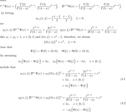
4.1. Case (i) λ= 0, kv= 0. The tempered fractional Dunkl operator acts on the functions Ψ and Θ
as follows:
Dα,λΨ(x) = Γ(3) Γ(3−α)x
2−α, Γ(4)
Γ(4−α)x
3−α; Dα,λΘ(x) = Γ(2)
Γ(2−α)x
1−α, Γ(3)
Γ(3−α)x
2−α.
Now, by letting
η1,2(x, ξ) = x−ξ
2 , x−ξ
2
, ξ= 0,
we have
η1(x, ξ).Dα,λΨ(x) =
x3−α Γ(3−α)+
3x4−α
Γ(4−α); η2(x, ξ).D
α,λΘ(x) = x 2−α
2Γ(2−α)+ x3−α Γ(3−α).
Considerρ1=ρ2= 1, x∈[0,1] andϑ(x, ξ) =x2−ξ, therefore, we obtain
kϑ(x, ξ)k2=x4, ξ= 0.
It is clear that
Ψ(ξ) = Ψ(0) = (0,0); Θ(ξ) = Θ(0) = (0,0),
then by assuming
φ1
Ψ(x)−Ψ(ξ)= 5x, φ2
Θ(x)−Θ(ξ)=−5x, x∈[0,1],
we conclude that
η1(x, ξ).DαΨ(x) +ρ1kϑ(x, ξ)k2=
x3−α
Γ(3−α)+
3x4−α
Γ(4−α)+x
4
<5x, x∈[0,1]
=φ1
Ψ(x)−Ψ(ξ)
(4.1)
and
η2(x, ξ).Dα,λΘ(x) +ρ2kϑ(x, ξ)k2=
x2−α
2Γ(2−α)+ x3−α
Γ(3−α)+x
4
<5x, x∈[0,1]
=−φ2
Θ(x)−Θ(ξ)
(4.2)
Hence, the couple (Ψ,Θ) is (α, λ, ρ, η, ϑ)-type univex atξ∈[0,1].Table 1 shows that for various values ofα∈(0,1),the outcomes yield the tempered fractional univexty of the couple (Ψ,Θ).
Table 1. Fractional multi-objective function,kv= 0
(α) Eq. (4.1) Eq. (4.2)
0.25 1.6 1.9
0.5 2.6 2.4
0.75 3.1 3.2
To apply the conditions of Theorem 3.1, we assume thatc1=c2= 1; thus, we havec1ρ1+c2ρ2= 2>0
with the inequalities (4.1) and (4.2). This leads that all the conditions of Theorem 3.1 are achieved and hence,ξ= 0 is an efficient solution. Note that if we letφ1(Y) = 3Y andφ2(Y) =−3Y,the couple
(Ψ,Θ) is not (α, λ, ρ, η, ϑ)-type univex atξ∈[0,1].
4.2. Case (ii) λ = 0, kv = 1. To evaluate the tempered fractional Dunkl operator, a calculation
implies that
σx2 =x2−2
v.x2
v.v =−x
2
, σx3 =−x3.
Therefore, one can attain
η1(x, ξ).Dα,λΨ(x) =
x3−α
Γ(3−α)+
x(2x2)α
2 +
3x4−α
Γ(4−α)+
x(2x3)α
and
η2(x, ξ).DαΘ(x) =
x2−α 2Γ(2−α)+
x(2x)α 2 +
x3−α Γ(3−α)+
x(2x2)α 2 .
Table 2 shows the evaluation of the tempered fractional multi-objective functions for different values ofα.
Table 2. Fractional multi-objective function,kv= 1
(α) Eq. (4.1) Eq. (4.2)
0.25 2.7 2.9
0.5 5 3.8
0.75 4.7 4.8
Thus, we conclude that the conditions of Theorem 3.1 are satisfied when c1 = c2 = 1; such that
c1ρ1+c2ρ2= 2>0 with the inequalities (4.1) and (4.2). Consequently, we obtainξ= 0 is an efficient
solution.
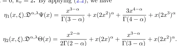
4.3. Case (iii) λ= 0, kv= 2. By applying (2.2), we have
η1(x, ξ).Dα,λΨ(x) =
x3−α
Γ(3−α)+x(2x
2)α+ 3x 4−α
Γ(4−α)+x(2x
3)α
and
η2(x, ξ).Dα,λΘ(x) =
x2−α
2Γ(2−α)+x(2x)
α+ x3−α
Γ(3−α)+x(2x
2)α.
Table 3 shows the evaluation of the tempered fractional multi-objective functions for different values of α.It is clear that the couple (Ψ,Θ) is not (α, λ, ρ, η, ϑ)-type univex at ξ∈[0,1].It is of (α, λ, ρ, η, ϑ)-type univex atξ∈[0,1],whenα∈(0,0.25].Hence, Theorem3.1can be applied only for this value of α.
Table 3. Fractional multi-objective function,kv= 2
(α) Eq. (4.1) Eq. (4.2)
0.25 3.5 4.1
0.5 5.4 5.2
0.75 6.4 5.5
4.4. Case (iv) λ= 1, kv = 0. The tempered fractional Dunkl operator acts on the functions Ψ and
Θ as follows:
Dα,λΨ(x) = Γ(3) Γ(3−α)x
2−α+x2ex, Γ(4)
Γ(4−α)x
3−α+x3ex;
Dα,λΘ(x) = Γ(2) Γ(2−α)x
1−α+xex, Γ(3)
Γ(3−α)x
2−α+x2ex.
Now, by letting
η1,2(x, ξ) = x−ξ
2 , x−ξ
2
, ξ= 0,
we have
η1(x, ξ).Dα,λΨ(x) =
x3−α Γ(3−α)+
x3ex 2 +
3x4−α Γ(4−α)+
x4ex 2 ;
η2(x, ξ).Dα,λΘ(x) =
x2−α
2Γ(2−α)+ x2ex
2 + x3−α
Γ(3−α)+ x3ex
2 .
Considerρ1=ρ2= 1, x∈[0,1] andϑ(x, ξ) =x2−ξ, therefore, we obtain
kϑ(x, ξ)k2=x4, ξ= 0.
It is clear that
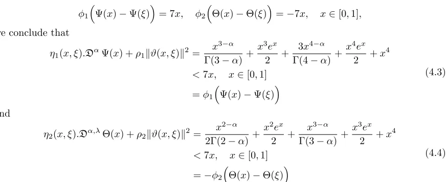
then by assuming
φ1
Ψ(x)−Ψ(ξ)= 7x, φ2
Θ(x)−Θ(ξ)=−7x, x∈[0,1],
we conclude that
η1(x, ξ).DαΨ(x) +ρ1kϑ(x, ξ)k2=
x3−α Γ(3−α)+
x3ex 2 +
3x4−α Γ(4−α)+
x4ex 2 +x
4
<7x, x∈[0,1]
=φ1
Ψ(x)−Ψ(ξ)
(4.3)
and
η2(x, ξ).Dα,λΘ(x) +ρ2kϑ(x, ξ)k2=
x2−α
2Γ(2−α)+ x2ex
2 + x3−α
Γ(3−α)+ x3ex
2 +x
4
<7x, x∈[0,1]
=−φ2
Θ(x)−Θ(ξ)
(4.4)
Hence, the couple (Ψ,Θ) is (α, λ, ρ, η, ϑ)-type univex atξ∈[0,1].Table 1 shows that for various values ofα∈(0,1),the outcomes yield the tempered fractional univexty of the couple (Ψ,Θ).
Table 4. ,kv= 0, λ= 1
(α,1) Eq. (4.3) Eq. (4.4)
0.25 4.3 4.6
0.5 5.4 5.1
0.75 5.8 5.9
To apply the conditions of Theorem3.1, we assume thatc1=c2= 1; thus, we havec1ρ1+c2ρ2= 2>0
with the inequalities (4.3) and (4.4). This leads that all the conditions of Theorem 3.1 are achieved and hence,ξ= 0 is an efficient solution. Note that if we letφ1(Y) = 5Y andφ2(Y) =−5Y,the couple
(Ψ,Θ) is not (α, λ, ρ, η, ϑ)-type univex atξ∈[0,1]. Also, the caseλ= 1 andkv = 1 does not imply
the univex function whenφ1(Y) = 7Y andφ2(Y) =−7Y.
5. Conclusion
This effort is generalized, for the first time, two important concepts in science. The Dunkl tempered fractional operator and the tempered Univex function, by utilizing the Caputo tempered fractional differential operator. These two generalizations are combined to deliver the fractional multi-objective problems. We studied the duality cases by minimize and maximize the desired function in theRn. Sim-ulation is provided to apply the existing solutions. It has been found that the fractional case converges to the ordinary case. These problems can be employed in many studies not only in mathematics, but also in the economy; such as the utility function the cost function and the entropy function.
References
[1] C.F. Dunkl, Differential-difference operators associated to reflection groups, Trans. Amer. Math. Soc. 311 (1) (1989), 167–183.
[2] M. Rosler and M. Voit, Markov processes related with Dunkl operators. Adv. Appl. Math. 21(4)(1998) 575–643. [3] R. W. Ibrahim, New classes of analytic functions determined by a modified differential-difference operator in a
complex domain, Karbala Int. J. Modern Sci. 3 (2017) 53–58.
[4] K.S. Miller, B. Ross, An Introduction to the Fractional Calculus and Fractional Differential Equations, John Wily& Sons (1993).
[5] A.A. Kilbas, H.M. Srivastava, J.J. Trujiilo, Theory and Applications of Fractional Differential Equations. Amster-dam, Netherlands: Elsevier (2006).
[6] B. Baeumer, M.M. Meerschaert, Tempered stable Levy motion and transient super-diffusion, J. Comput. Appl. Math. 233 (2010) 243–2448.
[7] R. W. Ibrahim, Fractional calculus of Multi-objective functions & Multi-agent systems. LAMBERT Aca- demic Publishing, Saarbrcken, Germany 2017.
[9] M.M. Meerschaert, A. Sikorskii, Stochastic Models for Fractional Calculus, De Gruyter, Berlin, 2012.
Faculty of Computer Science and Information Technology, University of Malaya, Malaysia