Radio Number for Fourth Power Paths

(1)

CSUSB ScholarWorks

Electronic Theses, Projects, and Dissertations Office of Graduate Studies

12-2014

Linda V. Alegria

California State University - San Bernardino

Follow this and additional works at: https://scholarworks.lib.csusb.edu/etd

Part of the Other Mathematics Commons

Recommended Citation Recommended Citation

Alegria, Linda V., "Radio Number for Fourth Power Paths" (2014). Electronic Theses, Projects, and Dissertations. 112.

https://scholarworks.lib.csusb.edu/etd/112

(2)

(3)

A Thesis

Presented to the

Faculty of

California State University,

San Bernardino

In Partial Fulfillment

of the Requirements for the Degree

Master of Arts

in

Mathematics

by

Linda Victoria Alegria

(4)

A Thesis

Presented to the

Faculty of

California State University,

San Bernardino

by

Linda Victoria Alegria

December 2014

Approved by:

Min-Lin Lo, Committee Chair Date

Joseph Chavez, Committee Member

Jeremy Aikin, Committee Member

Charles Stanton, Chair, Corey Dunn

Department of Mathematics Graduate Coordinator,

(5)

Abstract

A path on n vertices, denoted by Pn, is a simple graph whose vertices can be

ordered so that two vertices are adjacent if and only if they are consecutive in the order.

A fourth power path, P_n4, is obtained fromPnby adding edges between any two vertices,

u and v, whose distance in Pn, denoted bydPn(u, v), is less than or equal to four. The diameter of a graphG, denoteddiam(G) is the greatest distance between any two distinct

vertices of G. Aradio labeling of a graphG is a functionf that assigns to each vertex a

label from the set{0,1,2, ...}such that|f(u)−f(v)| ≥diam(G)−d(u, v)+1 holds for any

two distinct vertices, u and v inG (i.e., u, v∈ V(G)). The greatest value assigned to a

vertex byf is called thespanof the radio labeling f, i.e., spanf =max{f(v) :v∈V(G)}.

The radio number ofG, rn(G), is the minimum span off over all radio labelingsf of G.

(6)

Acknowledgements

I am indebted to my advisor, mentor, and supporter Dr. Min-Lin Lo for

provid-ing me not only with guidance and knowledge durprovid-ing this journey, but with invaluable

advice and words of wisdom. If it were not for her never-ending encouragement and

belief in me, I know I would not be where I am at today. I would also like to thank my

committee members, Dr. Joseph Chavez and Dr. Jeremy Aikin, for their assistance in

proof-reading the text and for their recommendations.

I owe special thanks to the program coordinator, Dr. Corey Dunn, as well as the

department chair, Dr. Charles Stanton. Only they know how much I have persistently

emailed them with my special concerns and requests. They have continuously assisted

me without hesitation. The Math Department also holds a special place as they have

always worked hard to support me during my entire academic career at CSUSB.

I also would like to thank my family: my mother Mirna Alegria, sister Lyzbeth

Alegria, brother David Alegria, and niece Katheryn Amaya for their love and support.

They have been my number-one fans, have shown me true unconditional love, and have

(7)

List of Tables

(10)

List of Figures

1.1 A graphG. . . 3

1.2 Simple graph vs. non-simple graph . . . 3

1.3 A graphGand a subgraph H of G . . . 4

1.4 A graphT . . . 4

1.5 Twoa−dwalks in T . . . 5

1.6 Distance betweenaand d . . . 5

1.7 Ana−f walk . . . 6

1.8 Diameter ofT . . . 6

1.9 P8 . . . 7

1.10 P8 vs. P84 . . . 7

1.11 Centers of odd and even paths . . . 8

1.12 Levels of vertices forneven andn odd . . . 9

1.13 Number line analogous to levels of Pn fornodd . . . 10

1.14 Number line vs. vertices on opposite sides of Pn fornodd . . . 11

1.15 Number line vs. vertices on opposite sides of Pn forneven . . . 12

1.16 First two vertices ofP7 labeled . . . 15

1.17 A radio labeling ofP7 with span equal to 36 . . . 15

1.18 v5 and v1 labeled in a radio labeling . . . 15

1.19 v5,v1 and v7 labeled in a radio labeling . . . 16

1.20 v5,v1,v7, andv4 labeled in a radio labeling . . . 16

1.21 A radio labeling ofP7 with span equal to 23 . . . 17

1.22 An optimal radio-labeling ofP7 . . . 17

1.23 P₈4 . . . 18

1.24 A radio labeling ofP4 8 with span equal to 14 . . . 19

1.25 A second radio labeling ofP₈4 with span equal to 14 . . . 19

1.26 A radio labeling ofP₈4 with span equal to 10 . . . 19

4.1 An optimal radio labeling ofP₁₈4 with span equal to 50 . . . 48

4.2 An optimal radio labeling ofP₁₉4 with span equal to 51 . . . 49

4.3 An optimal radio labeling ofP₂₀4 with span equal to 52 . . . 49

4.4 An optimal radio labeling ofP₂₁4 with span equal to 52 . . . 49

4.5 An optimal radio labeling ofP₂₂4 with span equal to 73 . . . 50

(11)

(12)

Chapter 1

Introduction

1.1

Channel Assignment Problem

Radio waves are a type of electromagnetic radiation. They have frequencies

from as little as three kHz, where one kHz is 1000 cycles per second, up to 300 GHz,

where one GHz is 1,000,000,000 cycles per second. Radio waves that are made

artifi-cially have many useful applications including radio communication, broadcasting, radar,

communications satellites and more. Depending on the frequency, radio waves behave

differently in the Earth’s atmosphere. Whether the wave travels to one general location

or whether it makes it across state lines depends on the length of the wave. In order

to avoid interference, the use of radio waves is controlled and monitored by law by the

International Telecommunications Union (ITU). In the United States, the Federal

Com-munications Commission (FCC) controls the use of specific frequencies and their purposes.

The radio spectrum is split up into radio bands based on frequency and is

des-ignated for different uses. AM radio stations, for instance, operate in a band of 535 kHz

to 1705 kHz. FM radio stations transmit radio waves in a band of frequencies between 88

MHz and 108 MHz. This band is further divided into 100 channels, each having a width

of 200 kHz, or 0.2 MHz. This is why your FM radio will be tuned in to a station with a

channel of 88.1, 88.3, 88.5, etc. For the most part, FM radio waves or signals travel in

a straight line, or are “line of sight”. The farther away from the FM station, the higher

(13)

lines, they can easily be interrupted by buildings, or other geographical structures such as

mountains. This would clearly explain why you would experience an interruption while

driving around mountains. It would make sense that the higher the FM transmitter

antennas are, the greater the area they will cover. There are more factors other than

antenna height that are involved in avoiding interference. One of the main factors is

dis-tance, namely the distance between the stations or transmitters. Since FM radio waves

are able to travel over limited distance, stations are able to share the same channel

pro-vided that they are at least a certain minimum distance apart. These stations would be

called co-channel stations. If restrictions on minimum distances are not met, the stations

would experience interference.

Generally speaking, stations are assigned channels based on their proximity to

one another. Stations that are closer to each other geographically must be assigned

chan-nels that have larger difference in value. Stations that have greater distance between

them can be assigned channels that are closer in value. The task of efficiently assigning

channels to radio transmitters is known as the Channel Assignment Problem. The Channel Assignment Problem became a problem of particular interest in the field of graph

theory since radio transmitters could be easily represented by vertices on a graph, and

distances between them could be represented by edges. There are different models that

have been inspired by the Channel Assignment Problem. We will later look at some

mod-els that were inspired by the Channel Assignment Problem after first covering some basics.

1.2

Basics of Graph Theory

In order to understand much of the language of this paper, let us define a few

basic terms and concepts concerning graphs.

A graph G consists of a finite, non-empty set V(G) of objects called vertices and a set E(G) of two-element subsets of V(G) called edges. The set V is called the vertex set of G, denotedV(G), and the set E is called the edge set of G, denoted E(G). If

(14)

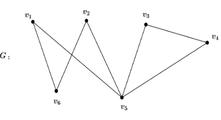
Figure 1.1 below is of a graphGwithV(G) ={v1, v2, v3, v4, v5, v6}andE(G) =

{v1v6, v1v5, v2v6, v2v5, v3v5, v3v4, v4v5}.

Figure 1.1: A graphG

A simple graphis a graph having no loops or multiple edges.

Figure 1.2: Simple graph vs. non-simple graph

The graphs mentioned in this paper will be simple graphs.

A subgraphof a graph G is a graph H such that the V(H) ⊆V(G) and the E(H) ⊆ E(G). The assignment of vertices to edges inH is the same as in G.

A walk in G is a sequence of vertices in G beginning with a vertex u and ending at some vertex v such that consecutive vertices in the sequence are adjacent. We can also

(15)

Figure 1.3: A graphG and a subgraphH of G

The length of a walk is the same as the number of edges traveled. In Figure 1.3 above, the length of thed−f walk,{d, c, e, f}, is three. Notice that thed−f walk,{d, c, e, f},

is not the shortest walk, or path in G from vertex d to vertex f. A shorter d−f walk

would be{d, c, f}, making the length of thatd−f walk equal to two.

In general, the distancebetween two verticesuandv of a graphG, denoted bydG(u, v)

or simply d(u, v) when the graph Gis clearly understood, is defined to be the minimum

length of any u−v walk. Moreover, the diameter of a graph G, denoted diam(G), is the greatest distance between any two vertices of G. In Figure 1.3, diam(G) is equal to

two.

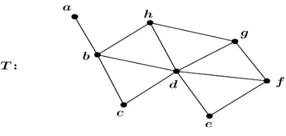
Figure 1.4: A graph T

(16)

vertices, distances between vertices, as well as the diameter of the graph.

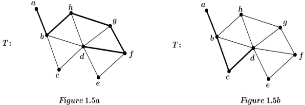
Figure 1.5: Twoa−dwalks in T

Now, in Figure 1.5a, the a−d walk is {a, b, h, g, f, d}. The length of thisa−dwalk is

five. In Figure 1.5b, the a−dwalk is {a, b, c, d}. The length of thisa−dwalk is three.

Now, with regard to the distance between aand d, the question becomes whether either

of these walks is the shortest possible walk in T. If there exists an a−dwalk of length

less than three, then three would not be the distance between vertices aand d.

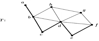
Figure 1.6: Distance betweena andd

Figure 1.6 shows an even shorter a−dwalk which is{a, b, d}. In this case, it is the most

direct and thus shortest a−dwalk inT. The length of this a−d walk is two, therefore

the distance between vertices a and d is equal to two. For fixed vertices u and v, there

may exist more than one walk in a graph whose length is equal to the distance between

u and v. In Figure 1.6, there happens to be one walk of minimum length from a to d.

(17)

distance between any two vertices of the graph. From the graph ofT, it seems as though

a andf may have the largest distance between them.

Figure 1.7: An a−f walk

In Figure 1.7, we have an a−f walk. We are seeking the diameter of graph

T and so we are looking at the maximum distance between any two vertices of T. The

length of the a−f walk is five. This, however is not the diameter of T. Again, the

diameter of T is the maximum distance among all distances between pairs of vertices in

T, not necessarily lengths of walks in T. The distance between a and f, in fact, is not

five.

Figure 1.8: Diameter of T

Now observe the a−f walk in Figure 1.8. Thisa−f walk has length equal to

three and is the shortest walk possible in T from a tof, therefore the distance between

aand f is equal to three . The diameter ofT,diam(T) actually turns out to be three as

well. In order to find the diameter of the graph, distances between all pairs of vertices

need to be considered, rather than arbitrary walks between vertices since these walks may

(18)

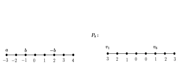
Apathis a simple graph whose vertices can be ordered so that two vertices are adjacent if and only if they are consecutive in the order.

Paths are denoted by Pn wheren is an integer and is equal to the number of vertices in

the path. Figure 1.9 is an example of P8, that is, a path on eight vertices.

Figure 1.9: P8

For a pathPn, the distance between any two vertices is equal to the number of

edges between them. Furthermore, the diameter of Pn is equal to the distance between

the first vertex and the last vertex. That is, diam(Pn) =n−1.

A graph Gis said to beconnected if there is a path between any pair of vertices ofG.

1.3

Fourth Power Paths

The main graph of interest in this paper is the fourth power path, denoted P_n4. A fourth power path, P_n4, is obtained from Pn by adding edges between vertices u and

v whose distance is at most four. Thus V(P_n4) is equal to V(Pn) and E(Pn4) is equal to

E(Pn)∪ {uv : 2≤d(u, v)≤4}. Figure 1.10 is an example ofP8 along withP84.

(19)

In this paper, we will denote the distance between vertices u and v of Pn by

dPn(u, v) and we will denote the distance between vertices uand v of P 4

n by d(u, v).

Recall that the distance between two vertices of a path is equal to the number

of edges between them. Also, notice that the distance between two adjacent vertices is

one, because there is one edge between any two adjacent vertices. For vertices u and v,

if dPn(u, v)≤4 then thed(u, v) = 1. Similarly, for vertices u and v, if 4< dPn(u, v)≤8 then the d(u, v) = 2. Furthermore, for vertices u and v, if 4(m−1) < dPn(u, v) ≤4m, m ∈N, then the d(u, v) =m. For this reason, the ceiling function is utilized in defining

the distance between any two vertices of P_n4.

Proposition 1.1. For any u, v∈V(P_n4), we have d(u, v) =

dPn(u, v) 4

This paper focuses entirely on fourth power paths, and so we will devote the

remainder of this section to explaining properties of Pn, which can further be extended

toP_n4, as well as defining terms that will be used throughout the paper.

We define a center of Pn as a vertex of Pn that is equidistant from both the

first vertex, v1, and the last vertex, vn, that is, the “middle vertex”. An odd path, Pn,

where n= 2m+ 1 for somem ∈_N will have only one center, namelyvm+1. A path, Pn,

where n= 2m for some m∈_Nwill have two centers, namely vm and vm+1. For n even, d(v1, vm) =d(vm+1, vn). Refer to Figure 1.11.

(20)

For each vertex u ∈ V(Pn), the level of u, denoted by L(u) is the smallest

distance in Pn from u to a center of Pn. The labeling of the levels can be viewed as

being analogous to labeling the number line with the exception of negative values. Levels

of vertices are greater than or equal to zero, where the only vertex whose level is equal

to zero is the center, or centers. Note that for P2m, there are two centers and thus two

vertices whose levels are equal to zero. Refer to Figure 1.12.

Figure 1.12: Levels of vertices for neven andnodd

For Pn, where n = 2m+ 1, L(v1) = m and L(vm+1) = 0. We will denote the

levels of a sequence of vertices A by L(A).

Ifn= 2m+ 1, then

L(v1, v2, ..., v2m+1) = (m, m−1, ...,3,2,1,0,1,2,3, ..., m−1, m).

Ifn= 2m, then

L(v1, v2, ..., v2m) = (m−1, m−2, ...3,2,1,0,0,1,2,3, ..., m−2, m−1).

Leftand rightvertices are defined as follows:

If n= 2m+ 1, then the left and right vertices, respectively are

(21)

If n= 2m, then the left and right vertices, respectively are

{v1, v2, ..., vm} and{vm+1, vm+2, ..., v2m}.

If two vertices are both right vertices or both left vertices, then we say that they are on

the same side. Otherwise, they are on opposite sides. Note that when n = 2m+ 1, the center is on both the right and the left side.

Paths have slightly different properties because of the parity ofn. Thus, we will

look at these two cases separately.

Let us investigate how the levels of vertices and the distances between them are

related. For each case, we will compare level sums of vertices to the respective values

found on the number line. Forn= 2m+ 1, there is only one center, thus only one vertex

with level equal to zero. When finding distances between two numbers or points,aandb,

on a number line, we simply compute|a−b|. Now, when two verticesuand vare on the

same side, we can find the distance between them, inP2m+1by doing the same operation

with the vertices’ respective levels.

Figure 1.13: Number line analogous to levels of Pn forn odd

In Figure 1.13, the distance between the points a and b is |a−b| which is

|(−3)−(−1)|and equals two. Looking atP7in Figure 1.13, the distance between vertices

v1 and v3 is also|L(v1)−L(v3)|which is|3−1|and equals 2. This is true whenever both

vertices, u and v are on the same side, that is dP2m+1(u, v) = |L(u)−L(v)|. Note that

(22)

We further investigate what would happen for vertices on opposite sides. On

the number line, finding the distance between two points aand b remains the same. It

is important to note, however, that when the two values have opposite signs, that is a

is positive and b is negative, when distance is calculated, the values are added. More

specifically, let a, b ∈ _N and consider −b. The distance between a and −b is |a−(−b)|

which is |a+b| and equals |a|+|b|. Thus the distance between two numbers a and b

is equal to the sum of their absolute values, only when aand b are on opposite sides of

the number line with respect to zero. We can apply this concept to the distance between

vertices u and v of P2m+1 when the vertices are on opposite sides. Refer to the Figure

1.14. The distance between points aand −bis | −3−1|which is | −4|and equals |3|+

|1|. In P7, the distance between v1 and v5 is |L(v1) +L(v5)| which is |3 + 1|and |3|+

|1|equals 4. Absolute value is not necessary when adding the levels of vertices since the

levels are always positive. Thus, for verticesuand vofP2m+1 that are on opposite sides, dP2m+1(u, v) =L(u) +L(v).

Figure 1.14: Number line vs. vertices on opposite sides of Pn forn odd

Now let us turn our attention toP2m, that is whennis even. The only difference

in the levels of vertices ofP2m is that there is an extra center, thus a second vertex whose

level is equal to zero. Finding the distance between vertices that are on the same side

remains equivalent to finding the distance between points on a number line. Therefore

we have dP2m(u, v) =|L(u)−L(v)| when u and v are vertices on the same side of P2m. Things change slightly when vertices u and v of P2m are on opposite sides. This case

becomes analogous to the number line, and to the case whennis odd, with the exception

of the extra center. Having an extra center adds an edge between the centers and thus

adds a distance of one to the distance between vertices on opposite sides.

(23)

Figure 1.15: Number line vs. vertices on opposite sides ofPn forneven

|a| + |b|. But the distance between v1 and v6 is not |L(v1) +L(v6)|. The extra edge

between the two centers must be taken into account. We fix this by simply adding one

to the level sums. That is, foru and v inP2m,dP2m(u, v) =L(u) +L(v) + 1 whenu and v are on opposite sides. Again, absolute value is not needed since the levels of vertices

are always positive. Recall that foru, v ∈P_n4,d(u, v) =ldPn(u,v) 4

m

.Combining this with

the observations above, we have the following:

Lemma 1.2. If n is odd, then for anyu, v∈V(P_n4), we have:

d(u, v) =

          

l_L₍_u₎₊_L₍_v₎

4

m

, if u and v are on opposite sides;

l_|

L(u)−L(v)|

4

m

, if u and v are on the same side.

If n is even, then for any u, v∈V(P4

n), we have:

d(u, v) =

          

l_L₍_u₎₊_L₍_v₎₊₁

4

m

, ifu andv are on opposite sides;

l_|

L(u)−L(v)|

4

m

, ifu andv are on the same side.

(See Appendix A.1 for proof of Lemma 1.2)

Due to the nature of the ceiling function, close and special attention needs to be

placed when adding or subtracting particular values prior to applying the ceiling function.

For example,₅₊₉

4

=₁₄

4

= 4.However,₅

4

+₉

4

= 2+3 = 5, thus ₅₊₉

4

6

=₅

4

+₉

4

(24)

Similarly, 10₄−5=5₄= 2.However, 10₄ −₅

4

= 3−2 = 1, thus 10₄−56=

₁₀

4

−₅

4

.This leads us to the following proposition, which we will make much use of

in later proofs.

Proposition 1.3. For any d1, d2 in N, we have:

d1+d2

4 =      l d1 4 m

+ld2

4

m

−1, if (d1, d2)≡4(1,1),(1,2),(1,3),(2,1),(2,2),(3,1);

l

d1

4

m

+ld2

4

m

, otherwise.

d1−d2

4 =      l d1 4 m

−ld2

4

m

+ 1, if (d1, d2)≡4(2,1),(3,1),(3,2),(0,1),(0,2),(0,3);

l

d1

4

m

−ld2

4

m

, otherwise.

More will be said about the level sums of vertices. First, let us briefly go over

radio labeling.

1.4

Radio Labeling

Motivated by the Channel Assignment Problem with only two levels of

inter-ference, a distance-two labeling (also called aλ-labeling andL(2,1)-labeling) for a graph Gis a function f :V(G)→ {0,1,2,3, ...}, where V(G) is the vertex set ofG such

that the following holds for all distinct u,v∈V(G):

|f(u)−f(v)| ≥

    

2, ifd(u, v) = 1;

1, ifd(u, v) = 2.

It is very important to note that there is no restriction for the labeling given to vertices

whose distance is strictly greater than two. This means that vertices whose distance is

greater than two are able to have the same label. Radio labeling extends the number of

interference levels considered in distance-two labeling from two, to the greatest distance

between any two vertices, that is, the diameter ofG. For a connected graphGof diameter

d, a radio labeling of G is a function f : V(G) → {0,1,2, ...} such that the following holds for any two distinct verticesu and v of G:

(25)

Note that in a radio labeling, restrictions are placed on every pair of vertices of G. If we

denote the last vertex labeled as xn, then f(xn) is the largest value assigned to a vertex

and thus is called the span of the radio labeling, i.e., spanf = max{f(v) : v ∈ V(G)}. The radio number of G, rn(G), is the minimum span off over all radio labelings f of

G. A radio labeling f ofGwithf(xn) = rn(G) is called aminimum radio labeling or

an optimal radio labeling.

We will now look at a few examples of radio labelings for a path on seven

ver-tices. It is important to understand that there is more than one way to label a graph, that

is, there are many radio labelings. There is, however, one radio number, which requires

a more specific, sometimes unique, labeling.

Before we attempt to labelP7, we determine the graph’s diameter. Since we are

dealing with a path, diam(P7) =d(v1, v7) = 6. Now, in order to obtain a radio labeling

of P7, it must be true that for any two distinct vertices of P7,d(u, v) +|f(u)−f(v)| ≥

1 +diam(P7), which impliesd(u, v) +|f(u)−f(v)| ≥7.Hence |f(u)−f(v)| ≥7−d(u, v).

This means that the difference in the values or labels of two vertices must be

greater than or equal to seven minus the distance between the two vertices. Now, for

the radio labeling, we can choose any vertex to begin with. We start with v1. We can

begin our labeling with any value, but in this paper we will always begin with zero.

Starting with zero makes calculating the span of the labeling much easier. The value

assigned to the next vertex in the labeling depends upon its distance from v1. If we

choose to simply label the vertices from left to right, and therefore label v2 next, we

must consider the distance between v1 and v2. We have d(v1, v2) = 1. Furthermore,

|f(u)−f(v)| ≥7−d(v1, v2) which implies|f(u)−f(v)| ≥7−1 = 6.

Therefore, the difference between the first label given tov1 and the second label

given to v2 must be at least six. Thus, v2 must be labeled six or any value larger than

six.

If we continue to label vertices from left to right, each new vertex will have a

label that is at least six greater than the previous vertex since the distance between each

(26)

Figure 1.16: First two vertices ofP7 labeled

Note that the span of the labeling in Figure 1.17 is 36.

Figure 1.17: A radio labeling ofP7 with span equal to 36

It is important to note that for the labeling to be a valid radio labeling,d(u, v) +

|f(u)−f(v)| ≥1 +diam(P7) needs to hold for all verticesuand v ofP7. We will take a

look at another labeling of P7. This time, we begin by labeling v5. Again, we will start

the labeling with zero. Next, we choose to label v1. The distance, d(v5, v1) = 4 so we

must obey the rule |f(v5)−f(v1)| ≥7−4 = 3.

Thus the difference between zero and the label given tov5must be at least three.

We will label v1 with three.

Figure 1.18: v5 and v1 labeled in a radio labeling

Next, we label the vertex,v7. Note thatd(v1, v7) = 6. Therefore, just as before,

(27)

Thus we will labelv7 with four.

Figure 1.19: v5,v1 and v7 labeled in a radio labeling

Again, it needs to be emphasized that|f(u)−f(v)| ≥1+diam(G)−d(u, v) needs

to hold for all vertices u andv ofG in order for the labeling to be a valid radio labeling.

For P7,|f(u)−f(v)| ≥ 7−d(u, v). We quickly verify whether this holds for verticesv5

and v7. The distance between the vertices, d(v7, v5) = 2, therefore, |f(v7)−f(v5)| ≥

7−2 and so|f(v7)−f(v5)| ≥5.

Thus the difference in labels given tov7andv5needs to be at least five. Therefore

we must either change the label given to v7 to five, or choose a different vertex to label.

For the labeling illustrated in Figure 1.20, we will simply change the label on v7 to five.

It is worth mentioning that what was done was considered a “jump” to the next integer

in order to satisfy the conditions of a radio labeling. Next we label v4. The distance

between v7 and v4, d(v7, v4) is three. As before, |f(v7)−f(v4)| ≥ 7−3 = 4 so we will

label v4 with nine. Once more, we must check that the appropriate condition holds for

v4 and v1, which it does.

Figure 1.20: v5,v1,v7, and v4 labeled in a radio labeling

We will continue by labeling the following vertices: v6, v2, andv3 respectively,

while making sure that the radio labeling condition is satisfied.

(28)

d(v6, v2) = 4 and so |f(v6)−f(v2)| ≥7−4 = 3,

d(v2, v3) = 1 and so |f(v2)−f(v3)| ≥7−1 = 6.

Again, we need to verify that the appropriate conditions are met for all vertices

of P7. So, in Figure 1.21 we have a radio labeling ofP7 with a span of 23.

Figure 1.21: A radio labeling ofP7 with span equal to 23

As we mentioned before, while there are many ways to give a valid radio labeling

of a graph, there is only one radio number and a special, many times unique, way to label.

Let us look at an optimal radio labeling of P7 in Figure 1.22. The span of P7 is equal to

rn(P7) which is 21.

Figure 1.22: An optimal radio-labeling ofP7

When looking to minimize the span, and in doing so, find the radio number of a

graphG, we want to label vertices in such a way that the distance between consecutively

labeled vertices is maximized. As we have seen, labeling vertices from left to right

defi-nitely does not achieve this because the distance between consecutively labeled vertices is

minimized. Starting on one side of the graph and then labeling vertices in an alternating

fashion seems to be a better choice since the distances between consecutively labeled

ver-tices almost stays constant and is not the minimum distance between verver-tices. Therefore

(29)

labeled vertices of a graph, and obtaining an optimal radio labeling of a graph.

The main topic of this paper concerns radio labelings of much more interesting

graphs. Namely, fourth power paths, denotedP_n4. Everything that we have covered thus far with regard to radio labeling will be dealt with in the same manner for P_n4 with the exception of the distances between vertices. Since P_n4 is obtained by adding edges between vertices of Pn that are distance four or less apart, the definition of distances

between vertices ofP_n4 is slightly altered. We must also keep in mind all of the properties of fourth power paths covered in the previous section. Thus, forP_n4, the following is true.

d(u, v) =

dPn(u, v) 4

u, v∈V(P_n4) (1)

diam(P_n4) =

n−1 4

(2)

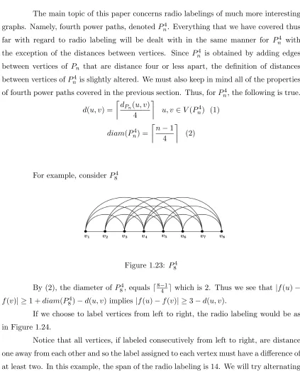
For example, consider P₈4

Figure 1.23: P₈4

By (2), the diameter of P₈4, equalsd8−₄1e which is 2. Thus we see that|f(u)−

f(v)| ≥1 +diam(P₈4)−d(u, v) implies|f(u)−f(v)| ≥3−d(u, v).

If we choose to label vertices from left to right, the radio labeling would be as

in Figure 1.24.

Notice that all vertices, if labeled consecutively from left to right, are distance

one away from each other and so the label assigned to each vertex must have a difference of

at least two. In this example, the span of the radio labeling is 14. We will try alternating

sides and see if this lowers the span.

The span of this labeling in Figure 1.25 was not reduced. This occurred because,

(30)

Figure 1.24: A radio labeling ofP₈4 with span equal to 14

Figure 1.25: A second radio labeling ofP₈4 with span equal to 14

labeling for each consecutively labeled vertex had to have a difference of at least two. In

order to reduce the span at all, the distance between at least one pair of consecutively

labeled vertices must be greater than one. We want to try to avoid consecutively labeling

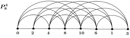
adjacent vertices as much as possible. Let us identify pairs of vertices u and v such

that the distance between them is strictly greater than one. Consider the following pairs

of vertices: {v1, v6},{v1, v7},{v1, v8},{v2, v7},{v2, v8}, and {v3, v8}. For these pairs of

vertices, the distance between them is strictly greater than one. The goal now becomes

to label these pairs of vertices consecutively in the labeling so that the difference in their

label will be at least one, rather than at least two. Observe the labeling of P8 in Figure

1.26.

(31)

The span of the labeling in Figure 1.26 was slightly reduced simply by

maximiz-ing distances between consecutively labeled vertices. Now,P₈4 was a rather simple fourth

power graph. For larger fourth power graphs, sayP4

25, labeling and obtaining an optimal

radio labeling becomes a much more complex task. A key component, however, has been

identified and that is that the distance between consecutively labeled vertices must be

maximized in order to reduce the span. In this paper, we will provide a lower bound

for the radio number of P_n4. Since, as we mentioned before, we approach P_n4 slightly differently depending on the parity of n, we will be considering two cases.

1.5

Notation and Labeling

Before we begin, it is important for the reader to understand much of the

nota-tion that is used in the labeling of P_n4 so we will define a few terms and notation first.

Let M, N ∈ N∪ {0}, then we define the ordered pair (M, N) to be a block, which

in-dicates a pattern to follow when labeling consecutive vertices. For example, if we begin

labeling using a (M, N) block, the first vertex labeled,xi, will have a level that is

con-gruent to M(mod p), where p is the power of the path. The next vertex labeled, xi+1,

will have a level that is congruent to N(modp). The following vertex labeled,xi+2, will

have level congruent to M(mod p), continuing in this fashion until all of the vertices of

levels congruent toM, N (modp) have been labeled. Labeling would then continue with

a new block with specified values. We may also choose to specify what side the vertex is

on by writing (LM, RN). This would mean that the first vertex labeled, xi, would be on

the left side and would have a level congruent to M(modp), then xi+1 would be on the

right side and would have a level congruent to N(mod p), so on and so forth. Without

loss of generality, in this paper, when labeling, blocks will always begin with vertices on

the left side of the graph. Since P_n4 is symmetric, beginning the labeling on the right side would behave in the same way as beginning on the left side.

A disconnection occurs (or we say that there is a disconnect) when L(xi) +L(xi+1)

is not congruent to a specified value modulo pthat maximizes the distance between two

(32)

case under consideration.

Disconnections will be ranked as being the best type, the second best type, the third best

type, ..., or the worst type of disconnection. The goal is to maximize distances between

consecutively labeled vertices. This is achieved by consecutively labeling vertices of

spe-cific levels or belonging to spespe-cific blocks until these vertices are exhausted, at which point

we have a disconnection. The worst type of disconnection is one which minimizes the

distance between the consecutively labeled vertices according to the respective level-sum

definition of distance.

A labeling pattern is a specific arrangement of blocks that specifies how vertices will be labeled.

For any labeling pattern, P_n4 will be said to have an “even” pairing if, for each block, (M, N), in the labeling pattern, the number of vertices with level congruent toM (mod

p) on one side equals the number of vertices with level congruent toN (modp) on the

other side. If the labeling of P_n4 does not have an “even” pairing, then P_n4 will be said to have extra vertices. These extra vertices, along with their respective levels, will be

closely noted, as they may end up altering the blocks in the labeling pattern. We will

(33)

Chapter 2

Lower Bound of rn

(

P

n

4

)

for

n

Even

2.1

General Lower Bound of rn

(

P

_n4

)

for

n

Even

Lemma 2.1 (General Lower Bound). Let P_n4 be a fourth power path on nvertices where n≥6 and let k=dn−₄1e, i.e., k=diam(P_n4).

If n is even, then rn(P_n4)≥

                

2k2_{+ 1}_, _if_n_≡ 80;

2k2, ifn≡82;

2k2+ 1, ifn≡₈4;

2k2, ifn≡86.

Proof of Lemma 2.1. Letfbe a radio-labeling forP_n4. Re-arrangeV(P_n4) ={x1, x2, ..., xn}

with 0 =f(x1)< f(x2)< f(x3)< ... < f(xn). Note that f(xn) is the span off.

By definition,f(xi+1)−f(xi)≥k+ 1−d(xi, xi+1) for 1≤i≤n−1. Summing

up these n−1 inequalities, we have

f(xn)≥(n−1)(k+ 1)− n−1

X

i=1

d(xi, xi+1).

Thus to minimize f(xn) it suffices to maximizePin=1−1d(xi, xi+1).

Since nis even,

n−1

X

i=1

d(xi, xi+1)≤

n−1

X

i=1

L(xi) +L(xi+1) + 1

4

.

(34)

1) For eachi, the equality ford(xi, xi+1) ≤

l_L₍_x

i)+L(xi+1)+1

4

m

holds only when xi and

xi+1 are on opposite sides, unless one of the vertices is a center and the other vertex

is of level not congruent to 0 (mod 4),

2) In the summationPn−1

i=1

l_L₍_x

i)+L(xi+1)+1

4

m

, each vertex of P_n4 occurs exactly twice, except for x1 andxn, for which each occurs only once.

By direct calculation (see Appendix A.2), we have

L(u) +L(v) + 1 4 =                 

L(u)+L(v)+4

4 , ifL(u) +L(v)≡4 0;

L(u)+L(v)+4

4 −

1

4, ifL(u) +L(v)≡4 1;

L(u)+L(v)+4

4 −

2

4, ifL(u) +L(v)≡4 2;

L(u)+L(v)+4

4 −

3

4, ifL(u) +L(v)≡4 3.

Therefore,

L(xi) +L(xi+1) + 1

4

≤ L(xi) +L(xi+1) + 4

4 ,

and the equality holds only ifL(xi) +L(xi+1)≡40. Combining this with 1) above, there

exist at most n−4 of the i0ssuch that d(xi, xi+1) = (L(xi) +L(xi+1) + 4)/4, i.e., there

are at least three disconnections in the labeling. Moreover, since among all the vertices

only the two centers are of level equal to zero, therefore L(x1) +L(xn) ≥0 + 0 = 0, we

conclude that

n−1

X

i=1

d(xi, xi+1)≤

"_n₋₁ X

i=1

L(xi) +L(xi+1) + 4

4 # −1 4− 1 4 − 1 4 = 1 4 " 2 n X i=1 L(xi)

!

−L(x1)−L(xn)

#

+ (n−1)−3

4 ≤ 1 4 " 2 n X i=1 L(xi)

!

−0−0

#

+ (n−1)− 3

4

= 1 2

h

20 + 1 + 2 +...+n 2 −1

i

+n−7

4

= n

2

8 +

3 4n−

7

4. (2.1)

Hence,

rn(P_n4)≥(n−1)(k+ 1)−

n2

8 +

3 4n−

7 4

(35)

There are four cases according ton(mod 8) whennis even. By direct calculation

(see Appendix B.1) and considering that rn(P_n4) is an integer, we have:

rn(P_n4)≥

                

2k2₊3 4

= 2k2_{+ 1}_, _if_n_≡

8 0 ( i.e.,n= 4k andk is even);

2k2−1₄

= 2k2, ifn≡8 2 ( i.e.,n= 4k−1 and kis odd);

2k2+3₄

= 2k2+ 1, ifn≡₈ 4 ( i.e.,n= 4k andk is odd);

2k2−1₄

= 2k2, ifn≡8 6 ( i.e.,n= 4k−2 and kis even).

Further investigation for a sharper lower bound of rn(P_n4) when n ≡8 4 and

when n≡₈ 6 is needed.

2.2

Sharper Lower Bound of rn

(

P

_n4

)

for the Case when

n

≡

4

or

6

(mod 8)

Lemma 2.2. LetP_n4 be a fourth power path onnvertices wheren≥6and letk=dn−₄1e, i.e., k=diam(P4

n).

rn(P_n4)≥

  

 

2k2+ 2, if n≡₈ 4;

2k2+ 1, if n≡8 6.

There are three cases to consider based on the number of disconnections that

occur in the labeling pattern. The types of disconnections will be investigated and looked

at in more detail in order to view the affects they have on the lower bound of rn(P4 8q+4)

and rn(P₈4_q₊₆).

Before we discuss the different cases, we must discuss the general labeling

tech-niques that will be applied. Recall that whennis even, in order to maximize the distance

between consecutively labeled vertices, the level sums of the consecutively labeled vertices

must be maximized as well. Therefore, we wish to label consecutive vertices xi and xi+1

(36)

xi+1, there is a disconnection in the labeling pattern whenever L(xi) +L(xi+1)6≡40.

Proof of Lemma 2.2. ForP_n4wherenis even, without consideration of any extra vertices, blocks in the labeling pattern will be of the following type (without loss of generality, we

start with a left vertex):

(L0, R0) (L1, R3) (L2, R2) (L3, R1)

We investigate separate cases based on the number of disconnections that occur in the

labeling pattern in the following subsections.

2.2.1 Case 1: At Least 5 Disconnections

There are at mostn−6 of thei0ssuch thatd(xi, xi+1) = (L(xi) +L(xi+1) + 4)/4.

That is, there are at least five disconnections in the labeling pattern andL(x1) +L(xn)≥

0 + 0 = 0.

Then,

n−1

X

i=1

d(xi, xi+1)≤

"_n₋₁ X

i=1

L(xi) +L(xi+1) + 4

4 # −1 4− 1 4 − 1 4 − 1 4 − 1 4 = 1 4 " 2 n X i=1 L(xi)

!

−L(x1)−L(xn)

#

+ (n−1)−5

4 ≤ 1 4 " 2 n X i=1 L(xi)

!

−0−0

#

+ (n−1)− 5

4

= 1 2

h

20 + 1 + 2 +...+n 2 −1

i

+n−9

4

= n

2

8 +

3 4n−

9

4. (2.2)

Note that Equation (2.2) is equal to Equation (2.1) minus 2₄.

Hence,

rn(P_n4)≥(n−1)(k+ 1)−

n2

8 +

3 4n−

9 4

.

(37)

rn(P_n4)≥                 

d(2k2₊3 4) +

2

4e= 2k2+ 2, ifn≡8 4

( i.e., n= 4kand kis odd);

d(2k2−1 4) +

2 4e= 2k

2_{+ 1}_, _if_n_≡ 8 6

( i.e., n= 4k−2 andk is even).

2.2.2 Case 2: Exactly 4 Disconnections

There are exactlyn−5 of thei0ssuch thatd(xi, xi+1) = (L(xi) +L(xi+1) + 4)/4,

that is, there are exactly four disconnections in the labeling pattern. This case will be

broken down into the following two sub-cases based on L(x1) +L(xn).

Case 2.1 L(x1) +L(xn)≥0 + 1 = 1, therefore

n−1

X

i=1

d(xi, xi+1)≤

"_n₋₁ X

i=1

L(xi) +L(xi+1) + 4

4 # −1 4 − 1 4 − 1 4− 1 4 = 1 4

"_n₋₁ X

i=1

L(xi) +L(xi+1)

#

+ (n−1)− 4

4 = 1 4 " 2 n X i=1 L(xi)

!

−L(x1)−L(xn)

#

+ (n−1)− 4

4 ≤ 1 4 " 2 n X i=1 L(xi)

!

−0−1 #

+ (n−1)−4

4

= 2 4

h

20 + 1 +...+n 2 −1

i

−1

4 + (n−1)− 4 4 = 1 2 2 n2 8 − n 4

+n−9

4

= n

2

8 +

3 4n−

9

4. (2.3)

Hence,

rn(P_n4)≥(n−1)(k+ 1)−

n2

8 +

3 4n−

9 4

(38)

Direct calculations (see Appendix B.3) lead to

rn(P_n4)≥

                

d(2k2+ 3₄) +2₄e= 2k2+ 2, ifn≡84

( i.e.,n= 4k andk is odd);

d(2k2− 1₄) +2₄e= 2k2+ 1, ifn≡86

( i.e.,n= 4k−2 and kis even).

Case 2.2 L(x1) +L(xn) = 0 + 0 = 0.

Claim: In this case, at least two of the disconnections that occur cannot be of the best type.

By direct calculation, our claim, and noting that L(x1) +L(xn) = 0 + 0 = 0, we

have,

n−1

X

i=1

d(xi, xi+1)≤

"_n₋₁ X

i=1

L(xi) +L(xi+1) + 4

4 # −1 4 − 1 4 − 2 4 − 2 4 = 1 4

"_n₋₁ X

i=1

L(xi) +L(xi+1)

#

+ (n−1)− 6

4 = 1 4 " 2 n X i=1 L(xi)

!

−L(x1)−L(xn)

#

+ (n−1)− 6

4 ≤ 1 4 " 2 n X i=1 L(xi)

!

−0−0

#

+ (n−1)−6

4

= 2 4

h

20 + 1 +...+n 2 −1

i

+ (n−1)−6

4 = 1 2 2 n2 8 − n 4

+n−10

4

= n

2

8 +

3 4n−

10

4 . (2.4)

Hence,

rn(P_n4)≥(n−1)(k+ 1)−

n2

8 +

3 4n−

10 4

(39)

By direct calculation (see Appendix B.3),

rn(P_n4)≥

        

       

d(2k2+ 3₄) +3₄e= 2k2+ 2, ifn≡₈4

( i.e.,n= 4k andk is odd);

d(2k2− 1 4) +

3 4e= 2k

2_{+ 1}_, _if_n_≡ 86

( i.e.,n= 4k−2 and kis even).

Proof of claim: For n ≡₈ 4 or 6, we have the following blocks as well as extra vertices:

(L0, R0), (L1, R3), (L2, R2), (L3, R1) L1, R1

We wish to have exactly four disconnections and we also want L(x1) +L(xn) =

0 + 0 = 0 under this case. Therefore we must break the (L0, R0) block in order to

begin with a vertex whose level is equal to zero and end with a vertex whose level

is equal to zero. Without considering any extra vertices for P₈4_q₊₄ and P₈4_q₊₆, we have the following blocks:

(L0, R0), (L1, R3) , (L2, R2) , (L3, R1), (L0, R0)

Note that any permutation of the above blocks will yield exactly four disconnections.

Now, P₈4_q₊₄ andP₈4_q₊₆ both have an extra set of vertices whose level is congruent to 1 (mod 4). We must arrange these vertices wisely in the labeling as to not increase

the number of disconnections that occur. Thus our new blocks become:

(L0, R0) , (L1, R3)-L1, (L2, R2) , R1-(L3, R1), (L0, R0)

Since we want L(x1) +L(xn) = 0 + 0 = 0, we must fix the (L0, R0) blocks so that

our labeling pattern starts and ends with the (L0, R0) blocks. Special attention is

given to the vertices whose levels are congruent to 1 (mod 4), that is, either the first

or the last vertex of the (L1, R3)−L1 or theR1−(L3, R1) blocks in the labeling

(40)

vertices and so all disconnections in the labeling pattern will occur at these “end

1” vertices. The best type of disconnection would occur if an “end 1” vertex was

followed or preceded by a vertex whose level was congruent to 0 (mod 4). However,

there are only two such vertices available. Therefore, at least two of the four “end

1” vertices cannot have disconnections of the best type.

Note: We can look at all possible permutations of the blocks for n even having 4

disconnections and look at all possible labeling patterns and observe that at least

two of the disconnections in the labeling patterns are indeed not of the best type.

Labeling pattern Disconnections Total

(0, 0) → (1, 3)-1 → (2, 2) → 1-(3, 1) → (0, 0) −1₄ −3₄ −3₄ −1₄ −8₄

(0, 0) → (1, 3)-1 → 1-(3, 1) → (2, 2) → (0, 0) −1 4 −

2 4 −

3 4 −

2

4 −

8 4

(0, 0) → (2, 2) → (1, 3)-1 → 1-(3, 1) → (0, 0) −2 4 −

3 4 −

2 4 −

1

4 −

8 4

Table 2.1: All labeling patterns for casesn≡4 or 6 (mod 8) with four disconnections

There are exactlyn−4 of thei0ssuch thatd(xi, xi+1) = (L(xi) +L(xi+1) + 4)/4,

that is, there are exactly three disconnections in the labeling pattern. Also note that

L(x1) +L(xn)≥0 + 1 = 1.

Claim: In this case, at least one of the disconnections in the labeling pattern will not be of the best type.

(41)

n−1

X

i=1

d(xi, xi+1)≤

"_n₋₁ X

i=1

L(xi) +L(xi+1) + 4

4 # −1 4− 1 4 − 2 4 = 1 4

"_n₋₁ X

i=1

L(xi) +L(xi+1)

#

+ (n−1)−4

4 = 1 4 " 2 n X i=1 L(xi)

!

−L(x1)−L(xn)

#

+ (n−1)−4

4 ≤ 1 4 " 2 n X i=1 L(xi)

!

−0−1 #

+ (n−1)−4

4 = 2 4 h 2

0 + 1 +...+

n

2 −1

i

−1

4 +n− 8 4 = 1 2 2 n2 8 − n 4

+n−9

4

= n

2

8 +

3 4n−

9

4. (2.5)

Hence,

rn(P_n4)≥(n−1)(k+ 1)−

n2

8 +

3 4n−

9 4

.

Direct calculations (see Appendix B.4) lead to,

rn(P_n4)≥

                

d(2k2+3₄) + 2₄e= 2k2+ 2, ifn≡₈ 4

( i.e., n= 4kand kis odd);

d(2k2−1 4) +

2 4e= 2k

2_{+ 1}_, _if_n_≡ 8 6

Proof of Claim :

For n≡₈ 4 or 6, we have the following blocks as well as extra vertices:

(L0, R0), (L1, R3), (L2, R2), (L3, R1) L1, R1

(42)

sides when labeling in order to achieve the best types of disconnects. To ensure that there

are only three disconnections, our new blocks must be:

(L0, R0) , (L1, R3)-L1, (L2, R2), R1-(L3, R1)

Observe that we have two blocks whose first and last vertex have level congruent to 1

(mod 4). Therefore there will be at least two disconnections that occur at these “end

1” vertices. The best case scenario consists of following or preceding each (1-(3-1)) or

((1-3)-1) block with a (L0, R0) block in the labeling to achieve disconnects of the best

type. This, however, is impossible to do without increasing the number of disconnections

that occur in the labeling. This means that at least one of the “end 1” vertices will have

to be followed or preceded by a vertex whose level is not congruent to 0 (mod 4) in the

labeling. If an “end 1” vertex is not followed or preceded by a vertex whose level is

con-gruent to 0 (mod 4), then it must be followed or preceded by a vertex whose level is either

congruent to 1 (mod 4) or congruent to 2 (mod 4). Thus, out of the three disconnections

that occur, at least two of them will occur at the “end 1” vertices. Furthermore, out of

these two disconnects that occur at the “end 1” vertices, at least one of them will not be

of the best type.

By Case 1, Case 2, and Case 3, we obtain the result stated in Lemma 2.2.

2.3

Summary of Results of Lower Bound of rn

(

P

_n4

)

for

n

Even

We have considered an arbitrary radio labeling ofP4

n forneven, having at least

3 disconnections, as well as further investigated special cases for n ≡₈ 4 and n≡₈ 6 in

order to obtain a sharper lower bound of rn(P_n4).

Combining Lemma 2.1 and Lemma 2.2, we have the following:

(43)

i.e., k=diam(P_n4).

If n is even, then rn(P_n4)≥

                

2k2+ 1, if n≡₈ 0;

2k2, if n≡8 2;

2k2+ 2, if n≡₈ 4;

2k2_{+ 1}_, _if _n_≡ 8 6.

Refer to Figures 4.1, 4.3, 4.5, and 4.7 for examples of radio labelings of P_n4 for

(44)

Chapter 3

Lower Bound of rn

(

P

n

4

)

for

n

Odd

3.1

Lower Bound of rn

(

P

_n4

)

for

n

Odd

Lemma 3.1. LetP_n4 be a fourth power path onnvertices wheren≥6and letk=dn−₄1e, i.e., k=diam(P_n4).

If n is odd, then rn(P_n4)≥

                        

2k2+ 2, if n≡81 and n≥17;

2k2+ 1, if n≡₈3;

2k2+ 2, if n≡85;

2k2+ 1, if n≡₈7;

2k2+ 1, if n= 9.

Proof of Lemma 3.1. We retain the same notation and employ the same method used in

the proof of Lemma 2.1. Since nis odd,

n−1

X

i=1

d(xi, xi+1)≤

n−1

X

i=1

L(xi) +L(xi+1)

4

.

Observe from the above inequality we have:

1) For each i, the equality for d(xi, xi+1) ≤

l_L₍_x

i)+L(xi+1)

4

m

holds only when xi and

xi+1 are on opposite sides, unless one of them is a center, and

2) In the summation Pn−1

i=1

l_L₍_x

i)+L(xi+1)

4

m

(45)

By direct calculation (see Appendix A.2), we have

L(u) +L(v) 4 =                 

L(u)+L(v)+3

4 −

3

4, ifL(u) +L(v)≡4 0;

L(u)+L(v)+3

4 , ifL(u) +L(v)≡4 1;

L(u)+L(v)+3

4 −

1

4, ifL(u) +L(v)≡4 2;

L(u)+L(v)+3

4 −

2

4, ifL(u) +L(v)≡4 3.

Therefore

L(xi) +L(xi+1)

4

≤ L(xi) +L(xi+1) + 3

4 ,

and the equality holds only if L(xi) +L(xi+1) ≡4 1. Combining this with 1), there are

two possible cases to consider, which will be covered in subsections 3.1.1 and 3.1.2.

3.1.1 Case 1: At Least 3 Disconnections

There exist at mostn−4 of thei0ssuch thatd(xi, xi+1) = (L(xi) +L(xi+1) + 3)/4. That

is, there are at least three disconnections in the labeling. In this case, since n is odd,

there is only one center. Therefore,L(x1) +L(xn)≥0 + 1 = 1.

Then

n−1

X

i=1

d(xi, xi+1)≤

"_n₋₁ X

i=1

L(xi) +L(xi+1) + 3

4 # −1 4− 1 4− 1 4 = 1 4 " 2 n X i=1 L(xi)

!

−L(x1)−L(xn)

#

+ 3

4(n−1)− 3 4 ≤ 1 4 " 2 n X i=1 L(xi)

!

−0−1

#

+3

4(n−1)− 3 4 = 2 4 2

1 + 2 + 3 +...+

n−1 2

−1

4 + 3 4n−

6 4 = n 2 8 + 3 4n−

15

8 . (3.1)

Thus,

rn(P_n4)≥(n−1)(k+ 1)−

n2

8 +

3 4n−

15 8

(46)

There are four cases according to n (mod 8) when n is odd. By direct calculation (see

Appendix C.1) and considering that rn(P_n4) is an integer, we have:

rn(P_n4)≥

        

       

2k2+ 1, ifn≡8 1 ( i.e.,n= 4k+ 1 and kis even);

d2k2+1₂e= 2k2+ 1, ifn≡₈ 3 ( i.e.,n= 4k−1 and kis odd);

2k2+ 1, ifn≡8 5 ( i.e.,n= 4k+ 1 and kis odd);

d2k2+1₂e= 2k2+ 1, ifn≡₈ 7 ( i.e.,n= 4k−1 and kis even).

Recall that when nis odd, the distance between consecutively labeled vertices,

xiandxi+1, is maximized whenL(xi) +L(xi+1)≡4 1. Also keep in mind that for vertices xi and xi+1, there is a disconnection in the labeling pattern whenL(xi) +L(xi+1)6≡41.

So the general blocks that must be used, without considering any extra vertices for a

particular case, are the following:

(L0, R1) (L1, R0) (L2, R3) (L3, R2)

We will investigate when there exist exactly n−3 of the i0s such that d(xi, xi+1) =

(L(xi) +L(xi+1) + 3)/4. That is, there are exactly two disconnections in the labeling. We

divide this discussion into two further sub-cases forn≡₈1 and then forn≡₈ 3,5, or 7. It

is recommended that the readers try a couple of examples to gain a better understanding

of the following claims.

If we wish to achieve a labeling pattern with only two disconnections, extra

attention must be placed on the positioning of the center, denoted by C, as to reduce the

number of disconnections by one.

Case 2.1: n≡1 (mod 8) If n≡₈ 1, then neitherx1 nor xn is the center. Therefore,

{L(x1), L(xn)} ≡4 {0,2},{0,3},{2,2}, or {3,3}. Note that for P84q+1 there is an

(47)

in order for there to be exactly two disconnections, we have the following blocks:

(L0, R1) - C - (L1, R0) (L2, R3) (L3, R2)

ThereforeL(x1) +L(xn)≥2 + 2 = 4. By similar calculation to Case 1, we have

n−1

X

i=1

d(xi, xi+1)≤

"_n₋₁ X

i=1

L(xi) +L(xi+1) + 3

4 # −1 4 − 1 4 = 1 4

"_n₋₁ X

i=1

L(xi) +L(xi+1)

#

+3

4(n−1)− 2 4 = 1 4 " 2 n X i=1 L(xi)

!

−L(x1)−L(xn)

#

+3

4(n−1)− 2 4 ≤ 1 4 " 2 n X i=1 L(xi)

!

−2−2 #

+3

4(n−1)− 2 4 = 2 4 2

1 + 2 +...+

n−1 2

−4

4 + 3

4(n−1)− 2 4 = 1 2 2 n2 8 − 1 8 +3 4n−

9 4 = n 2 8 + 3 4n−

19

8 . (3.2)

Therefore by direct calculations (see Appendix C.2), sincen= 4k+ 1 andkis even,

we have

rn(P_n4)≥

(2k2+ 1) + 3

4 − 1 4 =

2k2+3 2

= 2k2+ 2.

(48)

on different sides, in the labeling as to not increase the number of disconnections.

Therefore, the blocks become:

R1 - (L0, R1) - C - (L1, R0) - L1 (L2, R3) (L3, R2)

If n≡85, then {L(x1), L(xn)} ≡4{1,2} or{2,2}.

Now, P₈4_q₊₅ has two extra pairs of vertices whose levels are congruent to 1 (mod 4) and 2 (mod 4). Their placement in the labeling must be done in a way that does

not increase the number of disconnections that occur in the labeling. Thus we have

the following blocks:

R1 - (L0, R1) - C - (L1, R0) - L1 (L2, R3) -L2 R2 - (L3, R2)

Therefore, for n≡₈ 3,5, or 7,L(x1) +L(xn)≥1 + 2 = 3.

n−1

X

i=1

d(xi, xi+1)≤

"_n₋₁ X

i=1

L(xi) +L(xi+1) + 3

4 # −1 4 − 1 4 = 1 4

"_n₋₁ X

i=1

L(xi) +L(xi+1)

#

+3

4(n−1)− 2 4 = 1 4 " 2 n X i=1 L(xi)

!

−L(x1)−L(xn)

#

+3

4(n−1)− 2 4 ≤ 1 4 " 2 n X i=1 L(xi)

!

−1−2 #

+3

4(n−1)− 2 4 = 2 4 2

1 + 2 +...+

n−1 2

−3

4 + 3

4(n−1)− 2 4 = 1 2 2 n2 8 − 1 8 +3 4n−

8 4 = n 2 8 + 3 4n−

17

8 . (3.3)

Thus, by direct calculation (see Appendix C.2) we have,

Forn≡83, rn(Pn4)≥

2k2+ 1 2 +2 4 − 1 4 =

2k2+3 4

(49)

For n≡85, rn(Pn4)≥

2k2+ 1+2

4 − 1 4 =

2k2+5 4

.

Forn≡87, rn(Pn4)≥

2k2+ 1 2 +2 4 − 1 4 =

2k2+3 4

.

Thus we have,

rn(P_n4)≥

                              

2k2+3₄= 2k2+ 1, ifn≡8 3

( i.e., n= 4k−1 andk is odd);

2k2+5₄

= 2k2+ 2, ifn≡₈ 5

( i.e., n= 4k+ 1 and k is odd);

2k2+3₄

= 2k2+ 1, ifn≡₈ 7

Note that the lower bound of rn(P_n4) under Case 2 for n≡8 3 or 7 coincides with

the corresponding formulas in Case 1.

Now assume n ≡8 1 and n ≥ 17, that is, n = 4k+ 1, k is even and k ≥ 4.

Assume to the contrary that f(xn) = 2k2+ 1. Then only Case 1 is possible and all of the

following must hold:

1) {x1, xn}={v2k+1, v2k+2}or {v2k+1, v2k}

That is,{x1, xn}={center, a vertex right next to center}

2) f(xi+1) =f(xi) +k+ 1−d(xi, xi+1) for alli

3) For alli≥1, the two verticesxi and xi+1 are on opposites sides unless one of them

is the center.

(50)

By 1) and by symmetry, we can assume thatx1 =v2k+1, i.e.,x1 is the center. Note

that here, nis odd and sov2k+1 is the only center. Also,n= 4k+ 1 for some even k and k≥ 4. Excluding the center, there are 4k vertices in total with 2k vertices

on each side. In particular, there are k₂ many vertices whose level is congruent to 0 (mod 4), 1 (mod 4), 2 (mod 4), and 3 (mod 4) on each side. Since xn is either

v2korv2k+2 and both of these vertices have level equal to 1, xn is right next to the

center. By 2) and 3), the only three t0s in 4) must be k+ 1, 2k+ 1, and 3k+ 1.

For otherwise, there would be at least four t0s withL(xt) +L(xt+1) ≡4 0,2, or 3.

Therefore we have:

5)

L(xi)≡40 ifi∈ {1,3,5, ..., k+ 1,3k+ 2,3k+ 4, ...,4k} L(xi)≡41 ifi∈ {2,4,6, ..., k,3k+ 3,3k+ 5, ...,4k+ 1}

L(xi)≡42 ifi∈ {k+ 2, k+ 4, k+ 6, ...,2k,2k+ 3,2k+ 5, ...,3k+ 1} L(xi)≡43 ifi∈ {k+ 3, k+ 5, k+ 7, ...,2k+ 1,2k+ 2,2k+ 4, ...,3k}

That is, the labeling pattern is the following arrangement of blocks of vertices:

C-(1, 0) - (2, 3) - (3, 2) - (0, 1)

Claim: {vn, v1}={xk+1, x3k+2}(i.e.,v1 and vnare the last vertex whose level

is congruent to 0 (mod 4) in the (1, 0) block and the first vertex whose level is congruent

to 0 (mod 4) in the (0, 1) block)

Assuming this claim, we can further assume that vn = xk+1 and v1 = x3k+2.

The proof for the other case is symmetric and thus equivalent.

By 5), L(xk) =a≡41 and L(xk+2) =b≡42. By 2), 3), the fact that kis even, and our

(51)

f(xk+1)−f(xk) =k+ 1−

2k+a

4

=k+ 1−

2k 4 + la 4 m

(∵(2k, a)≡4 (0,1))

= k 2 + 1−

la

4

m

,

f(xk+2)−f(xk+1) =k+ 1−

b+ 2k

4

=k+ 1−

b 4 + 2k 4

(∵(b,2k)≡₄(2,0))

= k 2 + 1−

b 4 , and so,

f(xk+2)−f(xk) =k+ 2−

la 4 m − b 4 .

By definition and by Lemma 1.2,

f(xk+2)−f(xk)≥k+ 1−

_|

a−b|

4

.

Therefore,

k+ 2−la

4 m − b 4

≥k+ 1−

_|

a−b|

4

.

Thus,

|a−b|

4

≥la

4 m + b 4

−1.

Case 1: a≥b

Then by Proposition 1.3 and (a, b)≡4 (1,2),

_|

a−b|

4

=

a−b

4

=la 4 m − b 4

≥la

4 m + b 4

−1,

1≥2

b

4

.

(52)

Case 2: b≥a

Then by Proposition 1.3 and (b, a)≡4 (2,1),

_|

a−b|

4

=

b−a

4 = b 4

−la

4

m

+ 1≥la

4 m + b 4

−1,

2≥2la 4

m

, and thus a= 0,1,2,3, or 4.

This implies that a= 1 sincea≡4 1.

Thus, sincea= 1, we haveL(xk) = 1 which means that it is the left vertex that

is right next to the center since xk+1 =vn is a right vertex. Thus xk=v2k. In a similar

fashion, we will show that x3k+3 has level equal to one, is also right next to the center on

the right side, and thus is equal to v2k+2.

Recall that we let v1 =x3k+2 and so L(x3k+2) = 2k. By 5) L(x3k+1) =a≡4 2

and L(x3k+3) =b≡41.

f(x3k+2)−f(x3k+1) =k+ 1−

2k+a

4

=k+ 1−

2k 4 + la 4 m

(∵(2k, a)≡4 (0,2))

= k 2 + 1−

la

4

m

,

f(x3k+3)−f(x3k+2) =k+ 1−

b+ 2k

4

=k+ 1−

b 4 + 2k 4

(∵(b,2k)≡4 (1,0))

= k 2 + 1−

b 4 , and so,

f(x3k+3)−f(x3k+1) =k+ 2−

la 4 m − b 4 .

f(x3k+3)−f(x3k+1)≥k+ 1−

|a−b|

4

(53)

Therefore,

k+ 2−la

4 m − b 4

≥k+ 1−

_|

a−b|

4

.

Thus,

|a−b|

4

≥la

4 m + b 4

−1.

Case 1: a≥b

Then by Proposition 1.3 and (a, b)≡₄ (2,1),

|a−b|

4

=

a−b

4 = la 4 m − b 4

+ 1≥la

4 m + b 4

−1,

2≥2

b

4

, and thusb= 0,1,2,3, or 4.

This implies that b= 1 sinceb≡₄1.

Case 2: b≥a

Then by Proposition 1.3 and (b, a)≡4 (1,2),

_|

a−b|

4

=

b−a

4 = b 4

−la

4

m

≥la

4 m + b 4

−1,

1≥2la 4

m

,and thus a= 0.

This implies thata= 0 which cannot happen because a≡4 2.

Therefore,b= 1 =L(x3k+3) which implies that x3k+3 is the right vertex that is

right next to the center since x3k+2 =v1 is a left vertex. Therefore,x3k+3=v2k+2.

ByL(x1)+L(xn) = 0+1 = 1 under Case 1, without loss of generality we assume

L(x1) = 0 which means x1 is the center, andL(xn) = 1 which means xn is right next to

the center. Now, xn is a right vertex sincex3k+2 =v1 is a left vertex, and soxn=v2k+2.

This implies thatxn=v2k+2=x3k+3. Butn= 4k+1 so 4k+1 = 3k+3 implies thatk= 2.

Thus we have arrived at a contradiction because we started withk≥4.

(54)

Proof of claim: Suppose v1 6∈ {xk+1, x3k+2}, that is v1 is not the first vertex

of the (0,1) block nor the last vertex of a (1,0) block. We know thatL(v1) = 2k≡4 0.

This means that v1 is inside one of the (0,1) or (1,0) blocks.

Letv1 =xc for somecwhere xc−1 and xc+1 are both vertices on the right side. L(xc−1)≡4 L(xc+1)≡4 1. LetL(xc−1) =y andL(xc+1) =z. By 2),

f(xc)−f(xc−1) =k+ 1−

2k+y

4

=k+ 1−

2k

4

+ly 4

m

(∵(2k, y)≡₄ (0,1))

= k 2 + 1−

ly

4

m

.

f(xc+1)−f(xc) =k+ 1−

z+ 2k

4

=k+ 1−

lz 4 m + 2k 4

(∵(z,2k)≡₄(1,0))

= k 2 + 1−

lz

4

m

.

Therefore,

f(xc+1)−f(xc−1) =k+ 2−

ly

4

m

−lz

4

m

.

f(xc+1)−f(xc−1)≥k+ 1−

_|

z−y|

4

.

Therefore,

k+ 2−ly

4

m

−lz

4

m

≥k+ 1−

_|

z−y|

4

.

Thus,

|z−y|

4

≥ly

4 m + lz 4 m

−1.

Case 1: y≥z

Then by Proposition 1.3 and (y, z)≡4 (1,1),

_|

z−y|

4

=

y−z

4

=ly 4

m

−lz

4

m

≥ly

4

m

+lz 4

m

−1.

Therefore,

1≥2lz 4

m

Radio Number for Fourth Power Paths

CSUSB ScholarWorks

Table of Contents

List of Tables

Chapter 1

Basics of Graph Theory

Fourth Power Paths

Radio Labeling

Notation and Labeling

Chapter 2

Sharper Lower Bound of rn

Summary of Results of Lower Bound of rn

Chapter 3