Current Electricity

3.1 I

In Chapter 1, all charges whether free or bound, were considered to be at rest. Charges in motion constitute an electric current. Such currents occur naturally in many situations. Lightning is one such phenomenon in which charges flow from the clouds to the earth through the atmosphere, sometimes with disastrous results. The flow of charges in lightning is not steady, but in our everyday life we see many devices where charges flow in a steady manner, like water flowing smoothly in a river. A torch and a cell-driven clock are examples of such devices. In the present chapter, we shall study some of the basic laws concerning steady electric currents.

3.2 E

C

Imagine a small area held normal to the direction of flow of charges. Both the positive and the negative charges may flow forward and backward across the area. In a given time interval t, let q₊ be the net amount (i.e., forward minus backward) of positive charge that flows in the forward direction across the area. Similarly, let q_– be the net amount of negative charge flowing across the area in the forward direction. The net amount of charge flowing across the area in the forward direction in the time interval t, then, is q = q₊– q_–. This is proportional to t for steady current

CURRENT

Physics

94

and the quotient

q I

t

= (3.1)

is defined to be the current across the area in the forward direction. (If it turn out to be a negative number, it implies a current in the backward direction.)

Currents are not always steady and hence more generally, we define the current as follows. Let ∆Q be the net charge flowing across a cross-section of a conductor during the time interval ∆t [i.e., between times t and (t + ∆t)]. Then, the current at time t across the cross-section of the conductor is defined as the value of the ratio of ∆Q to ∆t in the limit of ∆t tending to zero,

( )

Q I t

t ∆ →

∆ ≡

∆ (3.2)

In SI units, the unit of current is ampere. An ampere is defined through magnetic effects of currents that we will study in the following chapter. An ampere is typically the order of magnitude of currents in domestic appliances. An average lightning carries currents of the order of tens of thousands of amperes and at the other extreme, currents in our nerves are in microamperes.

3.3 E

C

C

An electric charge will experience a force if an electric field is applied. If it is free to move, it will thus move contributing to a current. In nature, free charged particles do exist like in upper strata of atmosphere called the ionosphere. However, in atoms and molecules, the negatively charged electrons and the positively charged nuclei are bound to each other and are thus not free to move. Bulk matter is made up of many molecules, a gram of water, for example, contains approximately 1022 molecules. These molecules are so closely packed that the electrons are no longer attached to individual nuclei. In some materials, the electrons will still be bound, i.e., they will not accelerate even if an electric field is applied. In other materials, notably metals, some of the electrons are practically free to move within the bulk material. These materials, generally called conductors, develop electric currents in them when an electric field is applied.

If we consider solid conductors, then of course the atoms are tightly bound to each other so that the current is carried by the negatively charged electrons. There are, however, other types of conductors like electrolytic solutions where positive and negative charges both can move. In our discussions, we will focus only on solid conductors so that the current is carried by the negatively charged electrons in the background of fixed positive ions.

95

number of electrons travelling in any direction will be equal to the number of electrons travelling in the opposite direction. So, there will be no net electric current.

Let us now see what happens to such a piece of conductor if an electric field is applied. To focus our thoughts, imagine the conductor in the shape of a cylinder of radius R (Fig. 3.1). Suppose we now take two thin circular discs of a dielectric of the same radius and put positive charge +Q distributed over one disc and similarly –Q at the other disc. We attach the two discs on the two flat surfaces of the cylinder. An electric field will be created and is directed from the positive towards the

negative charge. The electrons will be accelerated due to this field towards +Q. They will thus move to neutralise the charges. The electrons, as long as they are moving, will constitute an electric current. Hence in the situation considered, there will be a current for a very short while and no current thereafter.

We can also imagine a mechanism where the ends of the cylinder are supplied with fresh charges to make up for any charges neutralised by electrons moving inside the conductor. In that case, there will be a steady electric field in the body of the conductor. This will result in a continuous current rather than a current for a short period of time. Mechanisms, which maintain a steady electric field are cells or batteries that we shall study later in this chapter. In the next sections, we shall study the steady current that results from a steady electric field in conductors.

3.4 O

’

L

A basic law regarding flow of currents was discovered by G.S. Ohm in 1828, long before the physical mechanism responsible for flow of currents was discovered. Imagine a conductor through which a current I is flowing and let V be the potential difference between the ends of the conductor. Then Ohm’s law states that

V ∝ I

or, V = R I (3.3)

where the constant of proportionality R is called the resistance of the conductor. The SI units of resistance is ohm, and is denoted by the symbol

Ω. The resistance R not only depends on the material of the conductor but also on the dimensions of the conductor. The dependence of R on the dimensions of the conductor can easily be determined as follows.

Consider a conductor satisfying Eq. (3.3) to be in the form of a slab of length l and cross sectional area A [Fig. 3.2(a)]. Imagine placing two such identical slabs side by side [Fig. 3.2(b)], so that the length of the combination is 2l. The current flowing through the combination is the same as that flowing through either of the slabs. If V is the potential difference across the ends of the first slab, then V is also the potential difference across the ends of the second slab since the second slab is

FIGURE 3.1 Charges +Q and –Q put at the ends of a metallic cylinder. The electrons will drift

because of the electric field created to neutralise the charges. The current thus will stop after a while unless the charges +Q

and –Q are continuously replenished.

FIGURE 3.2

Illustrating the relation R = ρl/A for

a rectangular slab of length l and area

Physics

96

identical to the first and the same current I flows through both. The potential difference across the ends of the combination is clearly sum of the potential difference across the two individual slabs and hence equals 2V. The current through the combination is I and the resistance of the combination R_C is [from Eq. (3.3)],

2 2 C V R R I

= = (3.4)

since V/I = R, the resistance of either of the slabs. Thus, doubling the length of a conductor doubles the resistance. In general, then resistance is proportional to length,

R l∝ (3.5)

Next, imagine dividing the slab into two by cutting it lengthwise so that the slab can be considered as a combination of two identical slabs of length l, but each having a cross sectional area of A/2 [Fig. 3.2(c)].

For a given voltage V across the slab, if I is the current through the entire slab, then clearly the current flowing through each of the two half-slabs is I/2. Since the potential difference across the ends of the half-slabs is V, i.e., the same as across the full slab, the resistance of each of the half-slabs R₁ is

1 2 2 .

( /2)

V V

R R

I I

= = = (3.6)

Thus, halving the area of the cross-section of a conductor doubles the resistance. In general, then the resistance R is inversely proportional to the cross-sectional area,

1 R

A

∝ (3.7)

Combining Eqs. (3.5) and (3.7), we have

l R

A

∝ (3.8)

and hence for a given conductor l

R A ρ

= (3.9)

where the constant of proportionality ρ depends on the material of the conductor but not on its dimensions. ρ is called resistivity.

Using the last equation, Ohm’s law reads I l

V I R A

ρ

= × = (3.10)

Current per unit area (taken normal to the current), I/A, is called current density and is denoted by j. The SI units of the current density are A/m2. Further, if E is the magnitude of uniform electric field in the conductor whose length is l, then the potential difference V across its ends is El. Using these, the last equation reads

GEORG SIMON OHM

(1787–

1

8

5

4

)

97

E l = j ρl

or, E = j ρ (3.11)

The above relation for magnitudes E and j can indeed be cast in a vector form. The current density, (which we have defined as the current through unit area normal to the current) is also directed along E, and is also a vector j (≡≡≡≡≡jE/E). Thus, the last equation can be written as,

E = jρ (3.12)

or, j = σE (3.13)

where σ ≡1/ρ is called the conductivity. Ohm’s law is often stated in an equivalent form, Eq. (3.13) in addition to Eq.(3.3). In the next section, we will try to understand the origin of the Ohm’s law as arising from the characteristics of the drift of electrons.

3.5 D

E

O

R

As remarked before, an electron will suffer collisions with the heavy fixed ions, but after collision, it will emerge with the same speed but in random directions. If we consider all the electrons, their average velocity will be zero since their directions are random. Thus, if there are N electrons and the velocity of the ith electron (i = 1, 2, 3, ... N) at a given time is v_i, then

1 1

0 N

i i

N

∑

Consider now the situation when an electric field is present. Electrons will be accelerated due to this field by

–e m

= E

a (3.15)

where –e is the charge and m is the mass of an electron. Consider again the ith electron at a given time t. This electron would have had its last collision some time before t, and let t_i be the time elapsed after its last collision. If v_iwas its velocity immediately after the last collision, then its velocity V_i at time t is

–

i i i

e t m

= E

V v (3.16)

since starting with its last collision it was accelerated (Fig. 3.3) with an acceleration given by Eq. (3.15) for a time interval t_i. The average velocity of the electrons at time t is the average of all the V_i’s. The average of v_i’s is zero [Eq. (3.14)] since immediately after any collision, the direction of the velocity of an electron is completely random. The collisions of the electrons do not occur at regular intervals but at random times. Let us denote by

τ, the average time between successive collisions. Then at a given time, some of the electrons would have spent

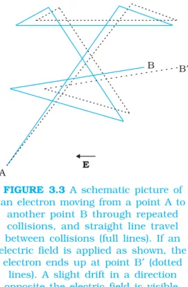
FIGURE 3.3 A schematic picture of an electron moving from a point A to

another point B through repeated collisions, and straight line travel between collisions (full lines). If an electric field is applied as shown, the

Physics

98

time more than τ and some less than τ. In other words, the time t_i in Eq. (3.16) will be less than τ for some and more than τ for others as we go through the values of i = 1, 2 ... N. The average value of t_i then is τ (known as relaxation time). Thus, averaging Eq. (3.16) over the N-electrons at any given time t gives us for the average velocity v_d

( )

( )

( )

d i _average i _average i _average e

t m

≡ = − E

v V v

0 –e e

m τ m τ

= E = − E (3.17)

This last result is surprising. It tells us that the electrons move with an average velocity which is independent of time, although electrons are accelerated. This is the phenomenon of drift and the velocity v_d in Eq. (3.17) is called the drift velocity.

Because of the drift, there will be net transport of charges across any area perpendicular to E. Consider a planar area A, located inside the conductor such that the normal to the area is parallel to E

(Fig. 3.4). Then because of the drift, in an infinitesimal amount of time ∆t, all electrons to the left of the area at distances upto |v_d|∆t would have crossed the area. If n is the number of free electrons per unit volume in the metal, then there are n ∆t |v_d|A such electrons. Since each electron carries a charge –e, the total charge transported across this area A to the right in time ∆t is –ne A|v_d|∆t. E is directed towards the left and hence the total charge transported along E across the area is negative of this. The amount of charge crossing the area A in time ∆t is by definition [Eq. (3.2)] I∆t, where I is the magnitude of the current. Hence,

d

I t∆ = +n e A v ∆t (3.18)

Substituting the value of |v_d| from Eq. (3.17)

2 e A

I t n t

m τ

∆ = ∆ E (3.19)

By definition I is related to the magnitude |j| of the current density by

I = |j|A (3.20)

Hence, from Eqs.(3.19) and (3.20),

2 ne

m τ

=

j E (3.21)

The vector j is parallel to E and hence we can write Eq. (3.21) in the vector form

2 ne

m τ

=

j E (3.22)

Comparison with Eq. (3.13) shows that Eq. (3.22) is exactly the Ohm’s law, if we identify the conductivity σ as

FIGURE 3.4 Current in a metallic conductor. The magnitude of current density in a metal is the magnitude of charge contained in a cylinder of unit

99

E

XAMPLE

3.1

2 ne

m

σ = τ (3.23)

We thus see that a very simple picture of electrical conduction reproduces Ohm’s law. We have, of course, made assumptions that τ and n are constants, independent of E. We shall, in the next section, discuss the limitations of Ohm’s law.

Example 3.1 (a) Estimate the average drift speed of conduction electrons in a copper wire of cross-sectional area 1.0 × 10–7 m2 carrying a current of 1.5 A. Assume that each copper atom contributes roughly one conduction electron. The density of copper is 9.0 × 103 kg/m3, and its atomic mass is 63.5 u. (b) Compare the drift speed obtained above with, (i) thermal speeds of copper atoms at ordinary temperatures, (ii) speed of propagation of electric field along the conductor which causes the drift motion.

Solution

(a) The direction of drift velocity of conduction electrons is opposite to the electric field direction, i.e., electrons drift in the direction of increasing potential. The drift speed v_dis given by Eq. (3.18)

v_d = (I/neA)

Now, e = 1.6 × 10–19 C, A = 1.0 × 10–7m2, I = 1.5 A. The density of conduction electrons, n is equal to the number of atoms per cubic metre (assuming one conduction electron per Cu atom as is reasonable from its valence electron count of one). A cubic metre of copper has a mass of 9.0 × 103 _{kg. Since 6.0 × 10}23 _copper atoms have a mass of 63.5 g,

23

6

6.0 10

9.0 10 63.5

n= × × ×

= 8.5 × 1028 m–3

which gives,

28 –19 –7

1.5

8.5 10 1.6 10 1.0 10

=

× × × × ×

d

v

= 1.1 × 10–3 _{m s}–1 _{= 1.1 mm s}–1

(b) (i) At a temperature T, the thermal speed* of a copper atom of mass M is obtained from [<(1/2) Mv2 > = (3/2) k_BT ] and is thus

typically of the order of k T M_B / _{, where} k_B is the Boltzmann constant. For copper at 300 K, this is about 2 × 102 m/s. This figure indicates the random vibrational speeds of copper atoms in a conductor. Note that the drift speed of electrons is much smaller, about 10–5 _{times the typical thermal speed at ordinary} temperatures.

(ii) An electric field travelling along the conductor has a speed of an electromagnetic wave, namely equal to 3.0 × 108 m s–1 (You will learn about this in Chapter 8). The drift speed is, in comparison, extremely small; smaller by a factor of 10–11.

Physics

100

E

XAMPLE

3.2

Example 3.2

(a) In Example 3.1, the electron drift speed is estimated to be only a few mm s–1 for currents in the range of a few amperes? How then is current established almost the instant a circuit is closed? (b) The electron drift arises due to the force experienced by electrons

in the electric field inside the conductor. But force should cause acceleration. Why then do the electrons acquire a steady average drift speed?

(c) If the electron drift speed is so small, and the electron’s charge is small, how can we still obtain large amounts of current in a conductor?

(d) When electrons drift in a metal from lower to higher potential, does it mean that all the ‘free’ electrons of the metal are moving in the same direction?

(e) Are the paths of electrons straight lines between successive collisions (with the positive ions of the metal) in the (i) absence of electric field, (ii) presence of electric field?

Solution

(a) Electric field is established throughout the circuit, almost instantly (with the speed of light) causing at every point a local electron

drift. Establishment of a current does not have to wait for electrons

from one end of the conductor travelling to the other end. However, it does take a little while for the current to reach its steady value. (b) Each ‘free’ electron does accelerate, increasing its drift speed until it collides with a positive ion of the metal. It loses its drift speed after collision but starts to accelerate and increases its drift speed again only to suffer a collision again and so on. On the average, therefore, electrons acquire only a drift speed.

(c) Simple, because the electron number density is enormous, ~1029 m–3.

(d) By no means. The drift velocity is superposed over the large random velocities of electrons.

(e) In the absence of electric field, the paths are straight lines; in the presence of electric field, the paths are, in general, curved.

3.5.1 Mobility

As we have seen, conductivity arises from mobile charge carriers. In metals, these mobile charge carriers are electrons; in an ionised gas, they are electrons and positive charged ions; in an electrolyte, these can be both positive and negative ions.

An important quantity is the mobility µ defined as the magnitude of the drift velocity per unit electric field:

| d| E

µ= v (3.24)

The SI unit of mobility is m2/Vs and is 104 of the mobility in practical units (cm2/Vs). Mobility is positive. From Eq. (3.17), we have

v_d = e E m

101

Hence,

d v e

E m

τ

µ = = (3.25)

where τ is the average collision time for electrons.

3.6 L

O

’

L

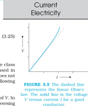
Although Ohm’s law has been found valid over a large class of materials, there do exist materials and devices used in electric circuits where the proportionality of V and I does not hold. The deviations broadly are one or more of the following types:

(a) V ceases to be proportional to I (Fig. 3.5).

(b) The relation between V and I depends on the sign of V. In other words, if I is the current for a certain V, then reversing the direction of V keeping its magnitude fixed, does not

produce a current of the same magnitude as I in the opposite direction (Fig. 3.6). This happens, for example, in a diode which we will study in Chapter 14.

(c) The relation between V and I is not unique, i.e., there is more than one value of V for the same current I (Fig. 3.7). A material exhibiting such behaviour is GaAs.

Materials and devices not obeying Ohm’s law in the form of Eq. (3.3) are actually widely used in electronic circuits. In this and a few subsequent chapters, however, we will study the electrical currents in materials that obey Ohm’s law.

3.7 R

V

M

The resistivities of various common materials are listed in Table 3.1. The materials are classified as conductors, semiconductors and insulators

FIGURE 3.5 The dashed line represents the linear Ohm’s law. The solid line is the voltage

V versus current I for a good conductor.

FIGURE 3.6 Characteristic curve of a diode. Note the different scales for negative and positive values of the voltage and current.

Physics

102

depending on their resistivities, in an increasing order of their values. Metals have low resistivities in the range of 10–8 Ωm to 10–6Ωm. At the other end are insulators like ceramic, rubber and plastics having resistivities 1018 times greater than metals or more. In between the two are the semiconductors. These, however, have resistivities characteristically decreasing with a rise in temperature. The resistivities of semiconductors are also affected by presence of small amount of impurities. This last feature is exploited in use of semiconductors for electronic devices.

T

3.1 R

Material Resistivity, ρ Temperature coefficient

(Ω m) at 0°C of resistivity, α(°C) –1

1 d

at 0 C dT

ρ

ρ  °

Conductors

Silver 1.6 × 10–8 0.0041

Copper 1.7 × 10–8 0.0068

Aluminium 2.7 × 10–8 0.0043

Tungsten 5.6 × 10–8 0.0045

Iron 10 × 10–8 0.0065

Platinum 11 × 10–8 0.0039

Mercury 98 × 10–8 0.0009

Nichrome ~100 × 10–8 0.0004

(alloy of Ni, Fe, Cr)

Manganin (alloy) 48 × 10–8 0.002 × 10–3

Semiconductors

Carbon (graphite) 3.5 × 10–5 – 0.0005

Germanium 0.46 – 0.05

Silicon 2300 – 0.07

Insulators

Pure Water 2.5 × 105

Glass 1010 – 1014

Hard Rubber 1013 – 1016

NaCl ~1014

Fused Quartz ~1016

103

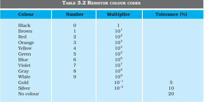
Resistors in the higher range are made mostly from carbon. Carbon resistors are compact, inexpensive and thus find extensive use in electronic circuits. Carbon resistors are small in size and hence their values are given using a colour code.

T

3.2 R

Colour Number Multiplier Tolerance (%)

Black 0 1

Brown 1 101

Red 2 102

Orange 3 103

Yellow 4 104

Green 5 105

Blue 6 106

Violet 7 107

Gray 8 108

White 9 109

Gold 10–1 5

Silver 10–2 10

No colour 20

The resistors have a set of co-axial coloured rings on them whose significance are listed in Table 3.2. The first two bands from the end indicate the first two significant figures of the resistance in ohms. The third band indicates the decimal multiplier (as listed in Table 3.2). The last band stands for tolerance or possible variation in percentage about the indicated values. Sometimes, this last band is absent and that indicates a tolerance of 20% (Fig. 3.8). For example, if the four colours are orange, blue, yellow and gold, the resistance value is 36 × 104Ω, with a tolerence value of 5%.

3.8

T

D

R

The resistivity of a material is found to be dependent on the temperature. Different materials do not exhibit the same dependence on temperatures. Over a limited range of temperatures, that is not too large, the resistivity of a metallic conductor is approximately given by,

ρ_T = ρ₀ [1 + α (T–T₀)] (3.26)

where ρ_T is the resistivity at a temperature T and ρ₀ is the same at a reference temperature T₀. α is called the temperature co-efficient of resistivity, and from Eq. (3.26), the dimension of α is (Temperature)–1.

FIGURE 3.8 Colour coded resistors (a) (22 × 102 Ω) ± 10%,

Physics

104

For metals, αis positive and values of α for some metals at T₀ = 0°C are listed in Table 3.1.

The relation of Eq. (3.26) implies that a graph of ρ_T plotted against T would be a straight line. At temperatures much lower than 0°C, the graph, however, deviates considerably from a straight line (Fig. 3.9).

Equation (3.26) thus, can be used approximately over a limited range of T around any reference temperature T₀, where the graph can be approximated as a straight line.

Some materials like Nichrome (which is an alloy of nickel, iron and chromium) exhibit a very weak dependence of resistivity with temperature (Fig. 3.10). Manganin and constantan have similar properties. These materials are thus widely used in wire bound standard resistors since their resistance values would change very little with temperatures.

Unlike metals, the resistivities of semiconductors decrease with increasing temperatures. A typical dependence is shown in Fig. 3.11.

We can qualitatively understand the temperature dependence of resistivity, in the light of our derivation of Eq. (3.23). From this equation, resistivity of a material is given by

2

1 m

n e ρ

σ τ

= = _(3.27)

ρ thus depends inversely both on the number n of free electrons per unit volume and on the average time τ between collisions. As we increase temperature, average speed of the electrons, which act as the carriers of current, increases resulting in more frequent collisions. The average time of collisions τ, thus decreases with temperature.

In a metal, n is not dependent on temperature to any appreciable extent and thus the decrease in the value of τ with rise in temperature causes ρ to increase as we have observed.

For insulators and semiconductors, however, n increases with temperature. This increase more than compensates any decrease in τ in Eq.(3.23) so that for such materials, ρ decreases with temperature.

FIGURE 3.9

Resistivity ρ_T of copper as a function

of temperature T.

FIGURE 3.10 Resistivity

ρT of nichrome as a function of absolute

temperature T.

FIGURE 3.11

Temperature dependence of resistivity for a typical

105

E

XAMPLE

3.4

Example 3.3 An electric toaster uses nichrome for its heating element. When a negligibly small current passes through it, its resistance at room temperature (27.0 °C) is found to be 75.3 Ω. When the toaster is connected to a 230 V supply, the current settles, after a few seconds, to a steady value of 2.68 A. What is the steady temperature of the nichrome element? The temperature coefficient of resistance of nichrome averaged over the temperature range involved, is 1.70 × 10–4 _°C–1_.

Solution When the current through the element is very small, heating effects can be ignored and the temperature T₁ of the element is the same as room temperature. When the toaster is connected to the supply, its initial current will be slightly higher than its steady value of 2.68 A. But due to heating effect of the current, the temperature will rise. This will cause an increase in resistance and a slight decrease in current. In a few seconds, a steady state will be reached when temperature will rise no further, and both the resistance of the element and the current drawn will achieve steady values. The resistance R₂ at the steady temperature T₂ is

R₂ 230 V 85.8

2.68 A

= = Ω

Using the relation

R₂ = R₁ [1 + α (T₂ – T₁)]

with α = 1.70 × 10–4 °C–1, we get

T₂ – T₁

–4

(85.8 – 75.3) (75.3) 1.70 10

=

× × = 820 °C

that is, T₂ = (820 + 27.0) °C = 847 °C

Thus, the steady temperature of the heating element (when heating effect due to the current equals heat loss to the surroundings) is 847 °C.

Example 3.4The resistance of the platinum wire of a platinum resistance thermometer at the ice point is 5 Ω and at steam point is 5.23 Ω. When the thermometer is inserted in a hot bath, the resistance of the platinum wire is 5.795 Ω. Calculate the temperature of the bath.

Solution R₀= 5 Ω, R₁₀₀= 5.23 Ω and R_t= 5.795 Ω

Now, 0 0

100 0

100, (1 )

t

t

R R

t R R t

R R α

−

= × = +

−

5.795 5 100 5.23 5

−

= ×

−

=0.795_0.23 ×100 = 345.65 °C

3.9 E

E

, P

Consider a conductor with end points A and B, in which a current I is flowing from A to B. The electric potential at A and B are denoted by V(A)

E

XAMPLE

Physics

106

and V(B) respectively. Since current is flowing from A to B, V(A) > V(B) and the potential difference across AB is V = V(A) – V(B) > 0.

In a time interval ∆t, an amount of charge ∆Q = I ∆t travels from A to B. The potential energy of the charge at A, by definition, was Q V(A) and similarly at B, it is Q V(B). Thus, change in its potential energy ∆U_pot is

∆U_pot = Final potential energy – Initial potential energy = ∆Q[(V (B) – V (A)] = –∆QV

= –I V∆t < 0 (3.28)

If charges moved without collisions through the conductor, their kinetic energy would also change so that the total energy is unchanged. Conservation of total energy would then imply that,

∆K = –∆U_pot (3.29)

that is,

∆K = I V∆t > 0 (3.30)

Thus, in case charges were moving freely through the conductor under the action of electric field, their kinetic energy would increase as they move. We have, however, seen earlier that on the average, charge carriers do not move with acceleration but with a steady drift velocity. This is because of the collisions with ions and atoms during transit. During collisions, the energy gained by the charges thus is shared with the atoms. The atoms vibrate more vigorously, i.e., the conductor heats up. Thus, in an actual conductor, an amount of energy dissipated as heat in the conductor during the time interval ∆t is,

∆W = I V∆t (3.31)

The energy dissipated per unit time is the power dissipated P = ∆W/∆t and we have,

P = I V (3.32)

Using Ohm’s law V = IR, we get

P = I 2R = V 2/R (3.33)

as the power loss (“ohmic loss”) in a conductor of resistance R carrying a current I. It is this power which heats up, for example, the coil of an electric bulb to incandescence, radiating out heat and light.

Where does the power come from? As we have reasoned before, we need an external source to keep a steady current through the conductor. It is clearly this source which must supply this power. In the simple circuit shown with a cell (Fig.3.12), it is the chemical energy of the cell which supplies this power for as long as it can.

The expressions for power, Eqs. (3.32) and (3.33), show the dependence of the power dissipated in a resistor R on the current through it and the voltage across it.

Equation (3.33) has an important application to power transmission. Electrical power is transmitted from power stations to homes and factories, which

FIGURE 3.12 Heat is produced in the resistor R which is connected across

the terminals of a cell. The energy dissipated in the resistor R comes from

107

may be hundreds of miles away, via transmission cables. One obviously wants to minimise the power loss in the transmission cables connecting the power stations to homes and factories. We shall see now how this can be achieved. Consider a device R, to which a power P is to be delivered via transmission cables having a resistance R_c to be dissipated by it finally. If V is the voltage across R and I the current through it, then

P = V I (3.34)

The connecting wires from the power station to the device has a finite resistance R_c. The power dissipated in the connecting wires, which is wasted is P_c with

P_c = I2R_c

2

2 c P R

V

= (3.35)

from Eq. (3.32). Thus, to drive a device of power P, the power wasted in the connecting wires is inversely proportional to V 2. The transmission cables from power stations are hundreds of miles long and their resistance R_c is considerable. To reduce P_c, these wires carry current at enormous values of V and this is the reason for the high voltage danger signs on transmission lines — a common sight as we move away from populated areas. Using electricity at such voltages is not safe and hence at the other end, a device called a transformer lowers the voltage to a value suitable for use.

3.10 C

R

– S

P

The current through a single resistor R across which there is a potential difference V is given by Ohm’s law I = V/R. Resistors are sometimes joined together and there are simple rules for calculation of equivalent resistance of such combination.

FIGURE 3.13 A series combination of two resistor R₁ and R₂.

Two resistors are said to be in series if only one of their end points is joined (Fig. 3.13). If a third resistor is joined with the series combination of the two (Fig. 3.14), then all three are said to be in series. Clearly, we can extend this definition to series combination of any number of resistors.

FIGURE 3.14 A series combination of three resistors R₁, R₂, R₃.

Two or more resistors are said to be in parallel if one end of all the resistors is joined together and similarly the other ends joined together (Fig. 3.15).

Physics

108

Consider two resistors R₁and R₂ in series. The charge which leaves R₁ must be entering R₂. Since current measures the rate of flow of charge, this means that the same current I flows through R₁ and R₂. By Ohm’s law:

Potential difference across R₁ = V₁ = I R₁, and

Potential difference across R₂ = V₂ = I R₂.

The potential difference V across the combination is V₁+V₂. Hence,

V = V₁+ V₂ = I (R₁ + R₂) (3.36)

This is as if the combination had an equivalent resistance R_eq, which by Ohm’s law is

R_eq V I

≡ = (R₁ + R₂) (3.37)

If we had three resistors connected in series, then similarly

V = I R₁ + I R₂ + I R₃ = I (R₁+ R₂+ R₃). (3.38) This obviously can be extended to a series combination of any number n of resistors R₁, R₂ ..., R_n. The equivalent resistance R_eq is

R_eq = R₁ + R₂ + . . . + R_n (3.39)

Consider now the parallel combination of two resistors (Fig. 3.15). The charge that flows in at A from the left flows out partly through R₁ and partly through R₂. The currents I, I₁, I₂ shown in the figure are the rates of flow of charge at the points indicated. Hence,

I = I₁ + I₂ (3.40)

The potential difference between A and B is given by the Ohm’s law applied to R₁

V = I₁R₁ (3.41)

Also, Ohm’s law applied to R₂ gives

V = I₂R₂ (3.42)

∴ I = I₁ + I₂ =

1 2 1 2

1 1

V V

V

R R R R

 

+ = _ + _

  (3.43)

If the combination was replaced by an equivalent resistance R_eq, we would have, by Ohm’s law

eq V I

R

= _(3.44)

Hence,

1 2

1 1 1

eq

R =R +R (3.45)

We can easily see how this extends to three resistors in parallel (Fig. 3.16).

109

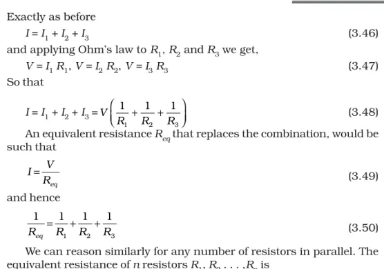
Exactly as before

I = I₁ + I₂ + I₃ (3.46)

and applying Ohm’s law to R₁, R₂ and R₃ we get,

V = I₁ R₁, V = I₂R₂, V = I₃R₃ (3.47) So that

I = I₁ + I₂ + I₃ =

1 2 3

1 1 1

V

R R R

 

+ +

 

  (3.48)

An equivalent resistance R_eq that replaces the combination, would be such that eq V I R = _(3.49) and hence

1 2 3

1 1 1 1

eq

R =R +R +R (3.50)

We can reason similarly for any number of resistors in parallel. The equivalent resistance of n resistors R₁, R₂ . . . ,R_n is

1 2 n

1 1 1 1

... eq

R =R +R + +R (3.51)

These formulae for equivalent resistances can be used to find out currents and voltages in more complicated circuits. Consider for example, the circuit in Fig. (3.17), where there are three resistors R₁, R₂ and R₃. R₂ and R₃are in parallel and hence we can

replace them by an equivalent 23

eq

R between point B and C with

23

2 3

1 1 1

eq R R

R = +

or, 23 2 3 2 3 Req R R R R = + (3.52)

The circuit now has R₁ and Req23 in series and hence their combination can be

replaced by an equivalent resistance R123eq

with

123 23 1

eq eq

R =R +R (3.53)

If the voltage between A and C is V, the current I is given by

(

)

123

1 2 3/ 2 3

eq

V V

I

R R R R R R

= =

 

+_ + _

(

)

1 2 1 3 2 3

V R R

R R R R R R

+ =

+ + (3.54)

FIGURE 3.17 A combination of three resistors R₁, R₂ and R₃. R₂, R₃ are in parallel with an equivalent resistance Req23. R1 and

23 eq

Physics

110

3.11 C

,

, I

R

We have already mentioned that a simple device to maintain a steady current in an electric circuit is the electrolytic cell. Basically a cell has two electrodes, called the positive (P) and the negative (N), as shown in Fig. 3.18. They are immersed in an electrolytic solution. Dipped in the solution, the electrodes exchange charges with the electrolyte. The positive electrode has a potential difference V₊ (V₊ > 0) between itself and the electrolyte solution immediately adjacent to it marked A in the figure. Similarly, the negative electrode develops a negative potential – (V_– ) (V_{– ≥} 0) relative to the electrolyte adjacent to it, marked as B in the figure. When there is no current, the electrolyte has the same potential throughout, so that the potential difference between P and N is V₊ – (–V_–) = V₊ + V_– . This difference is called the electromotive force (emf) of the cell and is denoted by ε. Thus

ε = V₊+V_–> 0 (3.55)

Note that ε is, actually, a potential difference and not a force. The name emf, however, is used because of historical reasons, and was given at a time when the phenomenon was not understood properly. To understand the significance of ε, consider a resistor R connected across the cell (Fig. 3.18). A current I flows across R from C to D. As explained before, a steady current is maintained because current flows from N to P through the electrolyte. Clearly, across the electrolyte the same current flows through the electrolyte but from N to P, whereas through R, it flows from P to N.

The electrolyte through which a current flows has a finite resistance r, called the internal resistance. Consider first the situation when R is infinite so that I = V/R = 0, where V is the potential difference between P and N. Now,

V = Potential difference between P and A + Potential difference between A and B + Potential difference between B and N

= ε (3.56)

Thus, emf ε is the potential difference between the positive and negative electrodes in an open circuit, i.e., when no current is flowing through the cell.

If however R is finite, I is not zero. In that case the potential difference between P and N is

V = V₊+ V_– – Ir

= ε – I r (3.57)

Note the negative sign in the expression (I r) for the potential difference between A and B. This is because the current I flows from B to A in the electrolyte.

In practical calculations, internal resistances of cells in the circuit may be neglected when the current I is such that ε >> I r. The actual values of the internal resistances of cells vary from cell to cell. The internal resistance of dry cells, however, is much higher than the common electrolytic cells.

FIGURE 3.18 (a) Sketch of an electrolyte cell with positive terminal P and negative terminal N. The gap between the electrodes is exaggerated for clarity. A

and B are points in the electrolyte typically close to

P and N. (b) the symbol for a cell, + referring to P and

– referring to the N electrode. Electrical connections to the cell are

111

We also observe that since V is the potential difference across R, we have from Ohm’s law

V = I R (3.58)

Combining Eqs. (3.57) and (3.58), we get I R = ε – I r

Or, I R r

ε

=

+ (3.59)

The maximum current that can be drawn from a cell is for R = 0 and it is I_max = ε/r. However, in most cells the maximum allowed current is much lower than this to prevent permanent damage to the cell.

C

In olden days lightning was considered as an atmospheric flash of supernatural origin. It was believed to be the great weapon of Gods. But today the phenomenon of lightning can be explained scientifically by elementary principles of physics.

Atmospheric electricity arises due to the separation of electric charges. In the ionosphere and magnetosphere strong electric current is generated from the solar-terrestrial interaction. In the lower atmosphere the current is weaker and is maintained by thunderstorm.

There are ice particles in the clouds, which grow, collide, fracture and break apart. The smaller particles acquire positive charge and the larger ones negative charge. These charged particles get separated by updrafts in the clouds and gravity. The upper portion of the cloud becomes positively charged and the middle negatively charged, leading to dipole structure. Sometimes a very weak positive charge is found near the base of the cloud. The ground is positively charged at the time of thunderstorm development. Also cosmic and radioactive radiations ionise air into positive and negative ions and air becomes (weakly) electrically conductive. The separation of charges produce tremendous amount of electrical potential within the cloud as well as between the cloud and ground. This can amount to millions of volts and eventually the electrical resistance in the air breaks down and lightning flash begins and thousands of amperes of current flows. The electric field is of the order of 105 V/m. A lightning flash is composed of a series of strokes with an average of about four and the duration of each flash is about 30 seconds. The average peak power per stroke is about 1012 watts.

Physics

112 E

XAMPLE

3.5

Example 3.5 A network of resistors is connected to a 16 V battery with internal resistance of 1Ω, as shown in Fig. 3.19: (a) Compute the equivalent resistance of the network. (b) Obtain the current in each resistor. (c) Obtain the voltage drops V_AB, V_BC and V_CD.

FIGURE 3.19

Solution

(a) The network is a simple series and parallel combination of resistors. First the two 4Ω resistors in parallel are equivalent to a resistor = [(4 × 4)/(4 + 4)] Ω = 2 Ω.

In the same way, the 12 Ω and 6 Ω resistors in parallel are equivalent to a resistor of

[(12 × 6)/(12 + 6)] Ω = 4 Ω.

The equivalent resistance R of the network is obtained by combining these resistors (2 Ω and 4 Ω) with 1 Ω in series, that is,

R = 2 Ω + 4 Ω + 1 Ω = 7 Ω.

(b) The total current I in the circuit is

16

2 A (7 1)

V I

R r ε

= = =

+ + Ω

Consider the resistors between A and B. If I₁ is the current in one of the 4 Ω resistors and I₂ the current in the other,

I₁ × 4 = I₂ × 4

that is, I₁ = I₂, which is otherwise obvious from the symmetry of the two arms. But I₁+ I₂ = I = 2 A. Thus,

I₁ = I₂ = 1 A

that is, current in each 4 Ω resistor is 1 A. Current in 1 Ω resistor between B and C would be 2 A.

Now, consider the resistances between C and D. If I₃ is the current in the 12 Ω resistor, and I₄ in the 6 Ω resistor,

I₃ × 12= I₄ × 6, i.e., I₄ = 2I₃

But, I₃ + I₄ = I = 2 A

Thus, I₃ = 2 3

   

  A, I4 =

4 3

      A

that is, the current in the 12 Ω resistor is (2/3) A, while the current in the 6 Ω resistor is (4/3) A.

(c) The voltage drop across AB is

VAB = I1 × 4 = 1 A × 4 Ω = 4 V,

113

E

XAMPLE

3.5

VAB = 2 A × 2 Ω = 4 V

The voltage drop across BC is

V_BC = 2 A × 1 Ω = 2 V

Finally, the voltage drop across CD is

V_CD = 12 Ω × I₃ = 12 Ω ×   _{ }2₃ A = 8 V.

This can alternately be obtained by multiplying total current between C and D by the equivalent resistance between C and D, that is,

V_CD = 2 A × 4 Ω = 8 V

Note that the total voltage drop across AD is 4 V + 2 V + 8 V = 14 V. Thus, the terminal voltage of the battery is 14 V, while its emf is 16 V. The loss of the voltage (= 2 V) is accounted for by the internal resistance 1 Ω of the battery [2 A × 1 Ω = 2 V].

3.12 C

S

P

Like resistors, cells can be combined together in an electric circuit. And like resistors, one can, for calculating currents and voltages in a circuit, replace a combination of cells by an equivalent cell.

FIGURE 3.20 Two cells of emf’s ε₁ and ε₂ in the series. r₁, r₂ are their internal resistances. For connections across A and C, the combination

can be considered as one cell of emf ε_eq and an internal resistance r_eq.

Consider first two cells in series (Fig. 3.20), where one terminal of the two cells is joined together leaving the other terminal in either cell free. ε₁, ε₂ are the emf’s of the two cells and r₁, r₂ their internal resistances, respectively.

Let V (A), V (B), V (C) be the potentials at points A, B and C shown in Fig. 3.20. Then V (A) – V (B) is the potential difference between the positive and negative terminals of the first cell. We have already calculated it in Eq. (3.57) and hence,

AB ( A) – (B) 1– 1

V ≡V V =ε I r (3.60)

Similarly,

BC (B) – (C) 2– 2

V ≡V V =ε I r (3.61)

Hence, the potential difference between the terminals A and C of the combination is

( )

( )

( )

( )

Physics

114

If we wish to replace the combination by a single cell between A and C of emf ε_eq and internal resistance r_eq, we would have

V_AC = ε_eq– I r_eq (3.63)

Comparing the last two equations, we get

ε_eq = ε₁ + ε₂ (3.64)

and r_eq = r₁ + r₂ (3.65)

In Fig.3.20, we had connected the negative electrode of the first to the positive electrode of the second. If instead we connect the two negatives, Eq. (3.61) would change to V_BC = –ε₂–Ir₂ and we will get

ε_eq = ε₁ – ε₂ (ε₁ > ε₂) (3.66) The rule for series combination clearly can be extended to any number of cells:

(i) The equivalent emf of a series combination of n cells is just the sum of their individual emf’s, and

(ii) The equivalent internal resistance of a series combination of n cells is just the sum of their internal resistances.

This is so, when the current leaves each cell from the positive electrode. If in the combination, the current leaves any cell from the negative electrode, the emf of the cell enters the expression for ε_eq with a negative sign, as in Eq. (3.66).

Next, consider a parallel combination of the cells (Fig. 3.21). I₁ and I₂ are the currents leaving the positive electrodes of the cells. At the point B₁, I₁ and I₂ flow in whereas the current I flows out. Since as much charge flows in as out, we have

I = I₁ + I₂ (3.67)

Let V (B₁) and V (B₂) be the potentials at B₁ and B₂, respectively. Then, considering the first cell, the potential difference across its terminals is V (B₁) – V (B₂). Hence, from Eq. (3.57)

( )

( )

V≡V B V B =ε I r (3.68)

Points B₁ and B₂ are connected exactly similarly to the second cell. Hence considering the second cell, we also have

( )

( )

V≡V B V B =ε I r (3.69)

Combining the last three equations

1 2

I = I + I

1 2 1 2

1 2 1 2 1 2

– – 1 1

–

V V

V

r r r r r r

ε ε ε ε   

= + =_ + _{ } + _

    (3.70)

Hence, V is given by,

1 2 2 1 1 2

1 2 1 2

–

r r r r

V I

r r r r

ε +ε

=

+ + (3.71)

If we want to replace the combination by a single cell, between B₁ and B₂, of emf ε_eq and internal resistance r_eq, we would have

V = ε_eq– Ir_eq (3.72)

FIGURE 3.21 Two cells in parallel. For connections

across A and C, the combination can be replaced by one cell of emf

ε_eq and internal resistances r_eq whose values are given in

115

The last two equations should be the same and hence

1 2 2 1

1 2 eq r r r r ε ε ε = + + (3.73) 1 2 1 2 eq r r r r r = + (3.74)

We can put these equations in a simpler way,

1 2 1 1 1

eq

r = +r r (3.75)

1 2

1 2 eq

eq

r r r

ε ₌ε ₊ε

(3.76)

In Fig. (3.21), we had joined the positive terminals together and similarly the two negative ones, so that the currents I₁, I₂ flow out of positive terminals. If the negative terminal of the second is connected to positive terminal of the first, Eqs. (3.75) and (3.76) would still be valid with ε 2 → –ε2

Equations (3.75) and (3.76) can be extended easily. If there an n cells of emf ε₁, . . . ε_nand of internal resistances r₁, . . . r_n respectively, connected in parallel, the combination is equivalent to a single cell of emf ε_eq and internal resistance r_eq, such that

1

1 1 1

eq n

r =r +L+r (3.77)

1

1

eq n

eq n

r r r

ε ₌ ε _{+ +} ε

L _(3.78)

3.13 K

’

R

Electric circuits generally consist of a number of resistors and cells interconnected sometimes in a complicated way. The formulae we have derived earlier for series and parallel combinations of resistors are not always sufficient to determine all the currents and potential differences in the circuit. Two rules, called Kirchhoff’s rules, are very useful for analysis of electric circuits.

Given a circuit, we start by labelling currents in each resistor by a symbol, say I, and a directed arrow to indicate that a current I flows along the resistor in the direction indicated. If ultimately I is determined to be positive, the actual current in the resistor is in the direction of the arrow. If I turns out to be negative, the current actually flows in a direction opposite to the arrow. Similarly, for each source (i.e., cell or some other source of electrical power) the positive and negative electrodes are labelled as well as a directed arrow with a symbol for the current flowing through the cell. This will tell us the potential difference, V = V (P) – V (N) = ε – Ir

Gustav Robert Kirchhoff (1824 – 1887) German physicist, professor at Heidelberg and at Berlin. Mainly known for his development of spectroscopy, he also made many important contributions to mathe-matical physics, among them, his first and second rules for circuits.

GUST

A

V

ROBER

T

Physics

116 E

XAMPLE

3.6

[Eq. (3.57) between the positive terminal P and the negative terminal N; I here is the current flowing from N to P through the cell]. If, while labelling the current I through the cell one goes from P to N, then of course

V = ε + Ir (3.79)

Having clarified labelling, we now state the rules and the proof:

(a) Junction rule: At any junction, the sum of the currents entering the junction is equal to the sum of currents leaving the junction (Fig. 3.22). This applies equally well if instead of a junction of several lines, we consider a point in a line.

The proof of this rule follows from the fact that when currents are steady, there is no accumulation of charges at any junction or at any point in a line. Thus, the total current flowing in, (which is the rate at which charge flows into the junction), must equal the total current flowing out.

(b) Loop rule: The algebraic sum of changes in potential around any closed loop involving resistors and cells in the loop is zero (Fig. 3.22). This rule is also obvious, since electric potential is dependent on the location of the point. Thus starting with any point if we come back to the same point, the total change must be zero. In a closed loop, we do come back to the starting point and hence the rule.

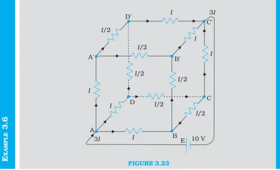
Example 3.6 A battery of 10 V and negligible internal resistance is connected across the diagonally opposite corners of a cubical network consisting of 12 resistors each of resistance 1 Ω (Fig. 3.23). Determine the equivalent resistance of the network and the current along each edge of the cube.

FIGURE 3.23 FIGURE 3.22 At junction a the current

leaving is I₁ + I₂ and current entering is I₃. The junction rule says I₃ = I₁ + I₂. At point h current entering is I₁. There is only one current leaving h and by junction rule that will also be I₁. For the loops ‘ahdcba’

117

E

XAMPLE

3.6

Solution The network is not reducible to a simple series and parallel combinations of resistors. There is, however, a clear symmetry in the problem which we can exploit to obtain the equivalent resistance of the network.

The paths AA′, AD and AB are obviously symmetrically placed in the network. Thus, the current in each must be the same, say, I. Further, at the corners A′, B and D, the incoming current I must split equally into the two outgoing branches. In this manner, the current in all the 12 edges of the cube are easily written down in terms of I, using Kirchhoff’s first rule and the symmetry in the problem.

Next take a closed loop, say, ABCC′EA, and apply Kirchhoff’s second rule:

–IR – (1/2)IR – IR + ε = 0

where R is the resistance of each edge and ε the emf of battery. Thus,

ε = 5 2I R

The equivalent resistance R_eq of the network is

5

3 6

eq

R R

I ε

= =

For R = 1 Ω, R_eq = (5/6) Ω and for ε = 10 V, the total current (= 3I) in the network is

3I = 10 V/(5/6) Ω = 12 A, i.e., I = 4 A

The current flowing in each edge can now be read off from the Fig. 3.23.

It should be noted that because of the symmetry of the network, the great power of Kirchhoff’s rules has not been very apparent in Example 3.6. In a general network, there will be no such simplification due to symmetry, and only by application of Kirchhoff’s rules to junctions and closed loops (as many as necessary to solve the unknowns in the network) can we handle the problem. This will be illustrated in Example 3.7.

Example 3.7 Determine the current in each branch of the network shown in Fig. 3.24.

FIGURE 3.24

Similation for application of Kirchhoff

ís

r

ules:

http://www.phys.hawaii.edu/~teb/optics/java/kirch3/

E

XAMPLE

Physics

118

E

XAMPLE

3.7

Solution Each branch of the network is assigned an unknown current to be determined by the application of Kirchhoff’s rules. To reduce the number of unknowns at the outset, the first rule of Kirchhoff is used at every junction to assign the unknown current in each branch. We then have three unknowns I₁, I₂ and I₃ which can be found by applying the second rule of Kirchhoff to three different closed loops. Kirchhoff’s second rule for the closed loop ADCA gives,

10 – 4(I₁– I₂) + 2(I₂ + I₃ – I₁) – I₁ = 0 [3.80(a)] that is, 7I₁– 6I₂ – 2I₃ = 10

For the closed loop ABCA, we get 10 – 4I₂– 2 (I₂ + I₃) – I₁ = 0

that is, I₁ + 6I₂ + 2I₃ =10 [3.80(b)]

For the closed loop BCDEB, we get 5 – 2 (I₂ + I₃) – 2 (I₂ + I₃ – I₁) = 0

that is, 2I₁ – 4I₂ – 4I₃ = –5 [3.80(c)]

Equations (3.80 a, b, c) are three simultaneous equations in three unknowns. These can be solved by the usual method to give

I₁ = 2.5A, I₂ = 5

8 A, I3 =

7 1

8 A

The currents in the various branches of the network are

AB : 5

8 A, CA : 1 2

2 A, DEB : 7 1

8 A

AD : 17

8 A, CD : 0 A, BC : 1 2

2 A

It is easily verified that Kirchhoff’s second rule applied to the remaining closed loops does not provide any additional independent equation, that is, the above values of currents satisfy the second rule for every closed loop of the network. For example, the total voltage drop over the closed loop BADEB

5 15

5 V 4 V 4 V

8 8

   

+_ × _ −_ × _

equal to zero, as required by Kirchhoff’s second rule.

3.14 W

B

As an application of Kirchhoff’s rules consider the circuit shown in Fig. 3.25, which is called the Wheatstone bridge. The bridge has four resistors R₁, R₂, R₃ and R₄. Across one pair of diagonally opposite points (A and C in the figure) a source is connected. This (i.e., AC) is called the battery arm. Between the other two vertices, B and D, a galvanometer G (which is a device to detect currents) is connected. This line, shown as BD in the figure, is called the galvanometer arm.

119

immediately gives us the relations I₁ = I₃ and I₂ = I₄. Next, we apply Kirchhoff’s loop rule to closed loops ADBA and CBDC. The first loop gives

–I₁R₁ + 0 + I₂R₂ = 0 (I_g = 0) (3.81)

and the second loop gives, upon using I₃ = I₁, I₄ = I₂

I₂R₄ + 0 – I₁R₃ = 0 (3.82)

From Eq. (3.81), we obtain,

1 2

2 1

I R I =R

whereas from Eq. (3.82), we obtain,

1 4

2 3

I R I =R

Hence, we obtain the condition

2 4

1 3

R R

R = R [3.83(a)]

This last equation relating the four resistors is called the balance condition for the galvanometer to give zero or null deflection.

The Wheatstone bridge and its balance condition provide a practical method for determination of an unknown resistance. Let us suppose we have an unknown resistance, which we insert in the fourth arm; R₄ is thus not known. Keeping known resistances R₁ and R₂ in the first and second arm of the bridge, we go on varying R₃ till the galvanometer shows a null deflection. The bridge then is balanced, and from the balance condition the value of the unknown resistance R₄ is given by,

2 4 3

1 R

R R

R

= _[3.83(b)]

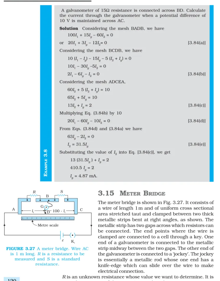
A practical device using this principle is called the meter bridge. It will be discussed in the next section.

Example 3.8 The four arms of a Wheatstone bridge (Fig. 3.26) have the following resistances:

AB = 100Ω, BC = 10Ω, CD = 5Ω, and DA = 60Ω.

FIGURE 3.26

FIGURE 3.25

E

XAMPLE

Physics

120

E

XAMPLE

3.8

A galvanometer of 15Ω resistance is connected across BD. Calculate the current through the galvanometer when a potential difference of 10 V is maintained across AC.

Solution Considering the mesh BADB, we have

100I₁ + 15I_g – 60I₂ = 0

or 20I₁ + 3I_g – 12I₂= 0 [3.84(a)]

Considering the mesh BCDB, we have

10 (I₁ – I_g) – 15I_g – 5 (I₂ + I_g) = 0

10I₁ – 30I_g –5I₂ = 0

2I₁ – 6I_g – I₂ = 0 [3.84(b)]

Considering the mesh ADCEA,

60I₂ + 5 (I₂ + I_g) = 10

65I₂ + 5I_g = 10

13I₂ + I_g = 2 [3.84(c)]

Multiplying Eq. (3.84b) by 10

20I₁ – 60I_g – 10I₂ = 0 [3.84(d)]

From Eqs. (3.84d) and (3.84a) we have

63I_g – 2I₂ = 0

I₂ = 31.5I_g [3.84(e)]

Substituting the value of I₂ into Eq. [3.84(c)], we get

13 (31.5I_g) + I_g = 2

410.5 I_g = 2

I_g = 4.87 mA.

3.15 M

B

The meter bridge is shown in Fig. 3.27. It consists of a wire of length 1 m and of uniform cross sectional area stretched taut and clamped between two thick metallic strips bent at right angles, as shown. The metallic strip has two gaps across which resistors can be connected. The end points where the wire is clamped are connected to a cell through a key. One end of a galvanometer is connected to the metallic strip midway between the two gaps. The other end of the galvanometer is connected to a ‘jockey’. The jockey is essentially a metallic rod whose one end has a knife-edge which can slide over the wire to make electrical connection.

R is an unknown resistance whose value we want to determine. It is connected across one of the gaps. Across the other gap, we connect a

FIGURE 3.27 A meter bridge. Wire AC is 1 m long. R is a resistance to be

121

standard known resistance S. The jockey is connected to some point D on the wire, a distance l cm from the end A. The jockey can be moved along the wire. The portion AD of the wire has a resistance R_cml, where R_cm is the resistance of the wire per unit centimetre. The portion DC of the wire similarly has a resistance R_cm (100-l).

The four arms AB, BC, DA and CD [with resistances R, S, R_cml and R_cm(100-l)] obviously form a Wheatstone bridge with AC as the battery arm and BD the galvanometer arm. If the jockey is moved along the wire, then there will be one position where the galvanometer will show no current. Let the distance of the jockey from the end A at the balance point be l=l₁. The four resistances of the bridge at the balance point then are R, S, R_cm l₁ and R_cm(100–l₁). The balance condition, Eq. [3.83(a)] gives

(

)

cm

R