Research of MDCOP Mining Based on Time Aggregated
Graph for Large Spatio-temproal Data Sets
Zhanquan Wang1,2, Taoli Han1, and Huiqun Yu1,2
1 Department of Computer Science and Engineering, East China University of Science and
Technology, Shanghai 200237, China
[email protected], [email protected], [email protected]
2
Shanghai Engineering Research Center of Smart Energy, Shanghai, 200237, China
Abstract. Discovering mixed-drove spatiotemporal co-occurrence patterns (MD-COPs) is important for network security such as distributed denial of service (DDoS) attack. There are usually many features when we are suffering from a DDoS attacks such as the server CPU is heavily occupied for a long time, bandwidth is hoovered and so on. In distributed cooperative intrusion, the feature information from multi-ple intrusion detection sources should be analyzed simultaneously to find the spatial correlation among the feature information.In addition to spatial correlation, intru-sion also has temporal correlation. Some invaintru-sions are gradually penetrating, and attacks are the result of cumulative effects over a period of time. So it is neces-sary to discover mixed-drove spatiotemporal co-occurrence patterns (MDCOPs) in network security. However, it is difficult to mine MDCOPs from large attack event data sets because mining MDCOPs is computationally very expensive. In informa-tion security, the set of candidate co-occurrence attack event data sets is exponential in the number of object-types and the spatiotemporal data sets are too large to be managed in memory. To reduce the number of candidate co-occurrence instances, we present a computationally efficient MDCOP Graph Miner algorithm by using Time Aggregated Graph. which can deal with large attack event data sets by means of file index. The correctness, completeness and efficiency of the proposed methods are analyzed.
Keywords:Network spatiotemporal co-occurrence pattern intrusion detection, mix-ed-drove spatiotemporal co-occurrence pattern, large spatiotemporal data set, Time Aggregated Graph (TAG), file index.
1.
Introduction
In network security area, intrusion detection is the detection of any intrusion that attempts to compromise the integrity, confidentiality, or availability of computer resources. Intru-sion detection collects and analyzes the information of key nodes in a computer network or system to detect the behaviors and signs of security policy violations and attacks in the network or system, and to respond accordingly.
points to invasion by the invasion of the source of the information is very fragmented, from a single intrusion detection information source may can’t see anything suspicious, cannot determine whether have intrusion behavior, only at the same time analysis of char-acteristic information from multiple source of intrusion detection, is likely to determine the intrusion behavior. The correlation between the feature information of this intrusion is called spatial co-occurrence.
In addition to spatial co-occurrence, intrusion also has temporal co-occurrence. Some invasions are gradually penetrating, and attacks are the result of cumulative effects over a period of time. Analysis from some intrusion behavior, for example, the characteristics of the information can be found that∆t period of network packet with the same source IP address, the address is trying to establish multiple connections with the same target host system. For this kind of intrusion behavior, if any time just thinks of this time period in isolation of characteristic information can reflect the attack, must consider all the feature information∆t period.
Intrusion detection which takes spatial and temporal into account is mixed-drove spa-tiotemporal co-occurrence patterns detection.
As the volume of spatiotemporal data continues to increase significantly due to both the growth of database archives and the increasing number of spatiotemporal sensors, au-tomatic and semi-auau-tomatic pattern analysis becomes more essential. It is meaningful and challenging for us to extract interesting patterns from these large spatiotemporal attack event data sets. Co-occurrence Pattern represents subsets of different object-types whose instances are co-located together for a significant fraction of time.
Given a large spatiotemporal attack event database, a neighbor relationship and mixed-drove interest measure thresholds, our aim is to discover mixed-mixed-drove spatiotemporal co-occurrence patterns (MDCOPs). To mine co-occurrence patterns, Celik et al. pro-posed MDCOP-Miner and fast MDCOP-Miner[14]. The two methods are based on the join-based collocation algorithm proposed by Huang et al.[18]. The basic co-occurrence pattern mining procedure involves four steps, as shown in Fig.1. First, candidate occurrence instances are gathered from the spatiotemporal data sets. Then, prevalent co-occurrence pattern sets satisfying the given prevalence thresholds are filtered. Finally, co-occurrence patterns satisfy the given prevalence thresholds are generated. Most of the computational time of co-occurrence pattern mining is devoted to finding co-occurrence instances. The approach is Apriori-like algorithm, which is costly as it enumerates all possible co-occurrence instances over all time instances. Thus, we propose adding a step for materializing the neighbor relationships to increase the efficiency of co-occurrence mining.
While the volume of the spatiotemporal data set is large, we find discovering the MD-COPs in a relatively small computer memory are difficult by using the existed methods. Mining the co-occurrence patterns is meaningful to network security.
1.1. Contributions
This study makes the following contributions:
This work provides a new storage method for mining MDCOPs from large spatiotem-poral attack data sets. The experimental results show that the proposed storage method and the pattern mining algorithms are correct, complete and efficient.
The framework of experimental design and the comparisons of existing approaches are provided in the paper.
Fig. 1. Basic procedure of co-occurrence pattern mining
1.2. Scope and Outline
This work is aim to addresses the co-occurrence pattern mining for large volume of spa-tiotemporal attack data sets. Our system achieves superior performance of computation efficiency to existing work like fast MDCOP-Miner [3]. Determining thresholds for MD-COP interest measures and inserting object-types at arbitrary time intervals are not the scope of this paper.
The rest part of this paper is organized as follows: Section 2 reviews related works. Section 3 presents basic concepts to provide a formal model of MDCOP Graph and the problem statement of mining MDCOPs. In Section 4, we presented our proposed MDCOP mining algorithms. Analysis of the algorithms is given in Section 5. Section 6 presents the experimental evaluation and section 7 presents conclusions and future work.
2.
Related Works
mixed object group [14]. However if there are no overlaps between the clusters in consec-utive time slots, their proposed algorithms for mining moving clusters will fail to discover MDCOPs.
The MDCOPs problem differs from the co-location pattern. Previous approaches of MDCOP mining can use a spatial co-location mining algorithm for each time slot to find spatial prevalent co-locations, and then apply a post-processing step to discover MD-COPs by check their time prevalence. To mine co-locations, Huang et al. firstly proposed the mining of co-location patterns(different subset of instances of object types are adja-cent to each other) from spatial datasets, then they proposed a join-based approach [20]; Cao et al. proposed a co-location approach from some period in spatiotemporal datasets, which can find out the co-location instances from continuous time slots [2]; Yoo et al. proposed a partial join-based and a join-less approach [18][11][12] which used nearby star and instance methods. Celik et al. [14]formalizes the problem, propose a new mono-tonic mixed-drove interest measure to discover and mine MDCOPs, and also propose an efficient algorithm (MDCOP-Miner).
MDCOPs represent object types co-located over space and time forming a spatial network (edges between objects in the network indicate existence of a neighborhood re-lationship) that dynamically changes over time. A common and naive approach to model such a network is to use time expanded graph, as described by Ko¨hler et al. [6] where the network is replicated across discrete time instants. Ding et al. [5] proposed an alternative approach where attributes at each node and edge of the graph are used to model state and topology changes respectively. A more efficient method of modeling temporal spatial networks was proposed by George et al. [7], by incorporating the properties of nodes and edges in the graph as a time series. This paper also proposed efficient algorithms for com-puting the shortest path and connectivity in time dependent networks modeled using time aggregated graphs. The problem of mining MDCOPs with high spatial and time preva-lence is described by Celik et al. [14]. However the approach is similar to Apriori like and involves candidate generation, which is costly as it enumerates all possible cliques over all time instances. A. Garaeva, M. Tang, Z. Wang, etc. [15][1] developed a frame-work implemented in Apache Spark environment for co-location patterns mining in big spatio-temporal data, which make evaluation of applied algorithms from the point of their efficiency and scalability.
Considerable achievements in MDCOP mining have been obtained in the last few years. However, dealing with large amount of spatiotemporal datasets is still challenging due to the accuracy and efficiency issues. In this paper, we materialize the neighbor re-lationships for efficient co-occurrence pattern mining, and solve the problem of efficient storage of MDCOPs by using the Time Aggregated Graph model and create our own storage model MDCOP Graph for mining MDCOPs. Finally, we provide an accurate and efficient co-occurrence pattern mining algorithm in large spatiotemporal datasets.
3.
Co-occurrence Pattern Mining
whether one pattern is co-occurrence pattern. Meanwhile, we use time aggregate graph as data storage structure.
3.1. Mixed-drove Prevalence Measure
The focus of this study is to mine MDCOPs with multiple prevalence measures from large spatiotemporal data sets. Co-occurrence pattern represents subsets of different object-types whose instance are located together for a significant fraction time. Mining occurrence patterns from spatiotemporal datasets is based on the mining of spatial co-location patterns from spatial datasets. Co-co-location pattern is the dataset of the frequent and closely adjacent spatial characteristics in the geographical space. Spatiotemporal co-occurrence patterns are the co-location patterns which satisfy the time prevalence mea-sure.
The basic MDCOP algorithm [14] defines two interest measures namely spatial preva-lenceθpand a time prevalence measureθtime.
The spatial prevalence measure is used to determine if the pattern is spatially prevalent in a specific time slot. The time prevalence measure is used to determine if the pattern is frequent in all time slots. These threshold values are mostly domain-specific. It is difficult to determine suitable interest measure thresholds to identify MDCOPs without domain knowledge. If the values of thresholds are too small, there are many unnecessary pat-terns will be generated. Otherwise, there are too few patpat-terns. It’s possible to miss some significant candidate MDCOPs if they are too large.
If a candidate pattern satisfies the following inequality, we can take this pattern as a spatial co-location pattern.
P robtmT F(s_prev(Pi, time_slot tm))≥θp (1)
Where,P rob(.)is the probability of overall prevalence time slots;s_prevstands for spa-tial prevalence measure;θpis the spatial prevalence measure. Hence, a pattern is defined
as an MDCOP if it satisfies the following inequality.
P robtmT F[s_prev(Pi, time_slot tm))≥θp]≥θtime (2) Where,P rob(.)is the probability of overall prevalence time slots;θpstands for spatial
prevalence measure;θtimeis the time prevalence measure. For example, in Fig. 2a, AB is
(a)
Mixed-Drove Spatial prevalence index values Time
Co-occurrence Patterns time slot() time slot1 time slot2 time slot3 prevalence index values
AB 3/5 3/5 3/5 3/5 4/4
AC 2/4 2/4 2/4 0 3/4
BC 0 3/5 3/5 3/5 3/4
ABC 0 2/5 2/5 0 2/4
(b)
Fig. 2.(a) An input spatiotemporal data set. (b) A set of output MDCOPs
Time Aggregated Graph (TAG) Spatiotemporal network is a spatial network whose topological relations and attribute information change with the passage of time. Spa-tiotemporal network model has many applications, such as real-time traffic planning, op-timal shortest path selection and so on. These applications need to create a spatiotemporal network model which can be queried and calculated efficiently.Kohler et al. proposes a spatiotemporal network model-time expanded graph. Spatial network for each time slot is established in this model, which results in a large duplication of node information. With the increase of time slots, the time-consuming of establishing time expanded graph also significantly increased. To solve this problem, George et al. proposes a more efficient method-time aggregate graph, which takes time series as the attribute of node and edge. The duplication problem is solved by using this method, while it is difficult to efficiently obtain the location relationships between target object and other objects in all time slots. Currently, modeling spatiotemporal objects by time aggregate graph is an ideal spatiotem-poral network model, which has low storage consumption, high query efficiency.
To take the advantage of time aggregate graph, we propose a graph based data struc-ture to capstruc-ture the information required to mine MDCOPs from the spatio-temoral data set. This data structure is motivated by Time Aggregated Graphs (TAG) [7] which models time varying road conditions as time series on the edges of a road network.[7] defines the time aggregated graph as follows.
T AG= (N, E, T F, f1...fk, g1...gm, w1...wp|fi:N→RT F;
gi:E→RT F;wi:E→RT F)
Where N is the set of nodes, E is the set of edges, TF is the length of the entire time interval,f1...fk are the mappings from nodes to nodes,g1...gmare mapping from edges
to edges, andw1...wpindicate the dependent weights (eg.travel times) on the edges.
Each edge has an attribute, called an edge time series that represents the time instants for which the edge is present. This enables TAG to model the topological changes of the network with time.
Fig. 3a, 3b, 3c shows a network at three time instants. The network topology and parameters change over time. For example, the edge N2-N1 is present at time slot 0, time slot 1 and disappears at time slot 2, and its weight changes from 1 at time slot 0 to 5 at time slot 1. The time aggregated graph that represents this dynamic network is shown in Fig. 3d. In this figure, edge N2-N1 has two attributes, each being a series. The attribute (0, 1) represents the time instants at which the edge is present and [1, 1, -] is the weight time series, indicating the weights at various instants of time.
TAG models the network which has topology change with time passage, it can stores and combines spatial and temporal information efficiently. Thus it can save a lot of mem-ory space and easily get all approaching slot information when querying examples of spatial relationships. Using the above-mentioned advantages of TAG model, we expand on this model and propose spatiotemporal co-occurrence storage model MDCOP Graph.
Fig. 3. (a), (b), (c) Network at various time instants. (d) Time Aggregated Graph (TAG). (e) Legend
3.2. Modeling MDCOP Graph
In this paper, we propose MDCOP Graph which based on TAG (Time Aggregated Graph) network model to store instances of close relationships, and obtain information for the process of mining co-occurrence patterns through visiting MDCOP Graph. Thus it can avoid a large number of join operations and complex space region split, which can im-prove the computational efficiency.
Given a set of spatiotemporal mixed object-types E, a neighborhood relation R, a set of time slots TF, a threshold pair (θp,θtime), MDCOP Graph can be represented as a
relationships. As we know that most of the computational time of co-occurrence pattern mining is devoted to finding co-occurrence instances. By means of MDCOP Graph, we don0t need to generate all possible candidate co-occurrence instances. We just generate real co-occurrence instances through visiting the MDCOP Graph. Thus, we can increase the efficiency of co-occurrence mining.
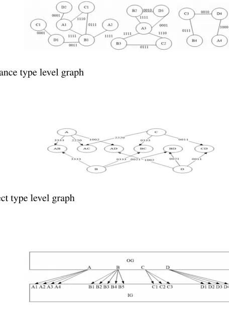
Definition 3.1 Given a set of co-occurrence instances CI, instance type level graph (IG) is used to captures the existence of co-location instances between two instance types over time. We define instance type level graph as follows.
IG= (I, CI, T F, f0...fk−1, e0...en−1,|fi:I→RT F;ei:CI→RT F) (4)
Where I is the set of instances of all object-types, CI is the set of co-location instances, TF is the length of the entire time interval, such that TF = [T0 ,...,Tn−1],f0...fk−1are
the mappings from object-types to object-types ,e0...en−1indicate the existence of
co-occurrence instances between two instance types over time on the edges.
For example, we generate instance type level graph (Fig.4) using the data set given in Fig. 2a. In Fig.4, we use time-series [1 1 1 0] to show that A1 and C1 are co-located at time slot 0, time slot 1, time slot 2 and disappear at time slot 3. Therefore, we can easily capture the existence of co-occurrence instances over time by traversing instance type level graph.
Definition 3.2 Given a set of candidate co-occurrence patterns (CP), object type level graph (OG) is used to indicate the participation count of particular object-types contribut-ing to particular co-occurrence patterns. We define object type level graph as follows.
OG= (E, CP, T F, f0...fk−1, p0...pn−1,|fi:ECPT F;pi:ECPT F) (5)
Where E is the set of spatiotemporal mixed object-types, CP is the set of co-occurrence patterns, TF is the length of the entire time interval,f0...fk−1are the mappings from
par-ticular object-types to the parpar-ticular co-occurrence patterns ,p0...pn−1indicate the
partic-ipation count of particular object-types contributing to particular co-occurrence patterns over time on the edges.
For example, we generate object type level graph (Fig.5) using the data set given in Fig. 2a. In Fig.2a, the co-occurrence pattern AC has co-occurrence instances sets A1, C1, A3, C2 at time slot 0, time slot 1 and time slot 2. At time slot 3, AC has no co-location instances. In Fig.5, since A1 and A3 are different instances of A, we used time-series [2 2 2 0] to show the participation count of object-type A contributing to co-location pattern AC. By using object type level graph, we can get the spatial prevalence index values and time prevalence index values.
Definition 3.3 Given instance type level graph and object type level graph, MDCOP Graph is composed of two parts: instance type level graph and object type graph. The instance type level and object type graphs are connected through links. We define MDCOP Graph as follows.
Where IG is instance type level graph, OG is object type level graph. TF is the length of the entire time interval, E is the set of spatiotemporal mixed object-types, I is the set of instances of all object-types.l0...lk−1are the mappings from object-types to their own
instances.
For example, we generate MDCOP graph (Fig.6) using the data set given in Fig. 2a. In Fig.6, both the instance type level and object type graphs are connected through links for easy traversal.
Fig. 4. Instance type level graph
Fig. 5.Object type level graph
Fig. 6. Object type level graph
3.3. Problem Statement
Given:
A set E of spatiotemporal object types over a common spatiotemporal framework. A neighbor relation R over locations.
A multiple set of user defined spatial and temporal prevalence thresholds.
Minimize cost of generate the MDCOP graph.
A set of frequent MDCOPs whose mixed-drove prevalence satisfies spatial and tem-poral prevalence thresholds.
Objective:
Capture and represent the temporal variation of MDCOPs. Minimize cost of candidate generation.
Minimize cost of generate the MDCOP graph.
Constraints:
To build the MDCOP graph that stores all the MDCOPs.
To find the correct and complete set of MDCOPs for any threshold value specified.
4.
Mining MDCOPS
In this section, we discuss fastMDCOP-Miner and then propose two novel MDCOP min-ing algorithms: MDCOP Graph Miner and LDMDCOP Graph Miner to mine MDCOPs. We also give the execution trace of these algorithms.
4.1. Fast MDCOP-Miner
FastMDCOP-Miner [3] uses a spatial co-location mining algorithm for each time slots to find spatial prevalent co-locations and prune time non-prevalent patterns as early as possible between the time slots to discover MDCOPs. To mine co-locations, Huang et al. proposed a join-based approach, Yoo et al. proposed a partial join-based approach and a join-less approach [16][18][11], this approach is based on the join-based collocation algorithm proposed by Huang et al., but it is also possible to use other approaches. Fast MDCOP-Miner [3] will first discover all size k spatial prevalent MDCOPs and prune time non-prevalent patterns as early as possible between the time slots to discover MDCOPs. Then the algorithm will generate size k +1 candidate MDCOPs using size k MDCOPs until there are no more candidates. However, this approach is Apriori like and involves candidate generation which is costly as it enumerates all possible cliques over all time instants.
4.2. MDCOP Graph Miner
To eliminate the drawbacks of fast MDCOP-Miner, we propose a MDCOP mining algo-rithm (MDCOP Graph Miner) to discover MDCOPs by storing all the MDCOPs in the MDCOP Graph.
Firstly, MDCOP Graph Miner will establish spatial temporal network MDCOP Graph, initialize the spatial relationship between each time slot; then it generates k+1 candidate spatiotemporal co-occurrence patterns; It obtains instance sets of candidate spatiotem-poral co-occurrence patterns through querying MDCOP Graph and calculates time and space frequent degrees, generate k+1 spatiotemporal co-occurrence patterns; Iteratively, it repeatedly generating candidate co-occurrence patterns until there is no new candidate co-occurrence pattern and algorithm terminate. Eventually, we get all the co-occurrence patterns meeting temporal and spatial thresholds.
We give the pseudo code of the algorithm and provide an execution trace of it using the data set in Fig. 2a. Algorithm1 shows the pseudo code of the MDCOP Graph Miner algorithm. This pseudo code is used to explain two algorithms: MDCOP Graph Miner and LDMDCOP Graph Miner which will be discussed in the next section. The choice of the algorithm is provided by the user. In the algorithm, steps 1-14 create the MDCOP Graph. Steps 15-21 give an iterative process to mine MDCOPs, steps 15-21 continue until there is no candidate MDCOP to be generated. Step 22 gives a union of the results. The execution traces of MDCOP Graph Miner are explained below.
Algorithm 1 pseudo code for the MDCOP Graph Miner Inputs:
E: a set of spatial object types
ST: a spatiotemporal data set < object_type, object_id, x, y, timeslot >
R: spatial neighborhood relationship TF: a time slot frame t0,...,tn−1
θ p:a spatial prevalence
θ time: a time prevalence threshold
Output: MDCOPs whose spatial prevalence indices, i.e., participation indices, are no less than θ p,
for time prevalence indices are no less than θ time. Variables:
t : time slots(t0,...,tn−1) k:co-occurrences size
Tk: set of instances of size k co-occurrences SPk: set of spatial prevalent size k co-occurrences TPk: set of time prevalent size k co-occurrences Ck: set of candidate size k co-occurrences MDPk: set of mixed-drove size k co-occurrences MDG: graph stores all the MDCOPs
Address: address for storing time series to the file Method:
k = 2
Ck (0) = gen_candidate_co_occ(E) for each time slot t in TF
Tk (t) = gen_co_occ_inst(Ck (t),ST, R) set timeSeries [t] =1 for Tk (t)
SPk (t) = find_spatial_prev_co_occ(Tk (t), θ p) TPk (t) = find_time_index(SPk (t))
MDPk (t) = find_time_prev_co_occ(TPk (t), θ time) Ck (t) = MDPk (t)
if(alg_choice "LDMDCOP Graph Miner")
Address = gen_co_occ_address (Tk (t) ) access the MDG file by the addresses
set timeSeries [t] =1 for Tk (t) if required if(alg_choice == "MDCOP Graph Miner")
while (not empty MDPk)
Ck +1 = gen _candidate_co_occ ( MDPk) Tk +1= gen _instancesTree (Ck +1,MDG) SPk+1 = find_spatial_prev_co_occ(Tk+1, θ p) TPk +1 = find_time_index(SPk+1 )
MDPk+1 = find_time_prev_co_occ(TPk+1, θ time) k = k+1
return union( MDP2 ,..., MDPk)
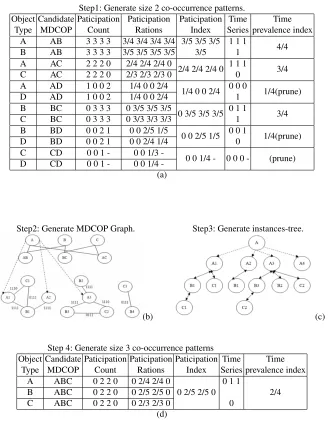
The execution trace of the MDCOP Graph Miner is given in Fig.7. This data set in Fig.2a. Contains four object-types A, B, C, and D and their instances in four time slots (i.e., A has four instances). The instances of each object-type have a unique identifier, such as A1. To discover MDCOPs, we use a monotonic composite interest measure which is a combination of the spatial prevalence and time prevalence measure. The spatial preva-lence measure shows the strength of the spatial co-location when the index is greater than or equal to a given threshold [3][18].The time prevalence measure shows the frequency of the pattern over time.
In step1, by dividing each entry in Fig. 7a with the corresponding number of instances for an object, we get the participation ratio of an object type in co-location. For example, the participation index of collocation AB is [3/5 3/5 3/5 3/5], which is the minimum par-ticipation ratio of type A and B in all time slots. We prune time non-prevalent patterns whose participation indices are less than a given threshold as early as possible. For exam-ple, there are four time slots and the time prevalence threshold is 0.5.In this case, a size k pattern should be present for at least two time slots to satisfy the threshold. If the time prevalence index of a pattern is 0 for the first (or any) three time slots, there is no need to generate it and check its prevalence for the rest of the time slots even if it is time persistent for the remaining time slots. Spatial prevalent patterns AB, AC, and BC are selected as MDCOPs since they are time prevalent (their time prevalence indices satisfy the given time prevalence threshold 0.5). In contrast, spatial prevalent patterns AD, BD and CD are pruned since they are time non-prevalent.
In step2, three sub-graphs on the bottom of Fig. 7b are created. It also creates links from the instance types to the object type, for example, Link between A3 and A if A3 is part of at least one co-occurrence. The links between the object and the instance type help in traversing the data set efficiently to calculate the spatial prevalence index values. Connections between the object type graph and the instance type graph are missing to reduce clutter and the series in the object graph has not been represented for the same reason. After the algorithm has been executed, the series on edge A and AB would be [3/4 3/4 3/4 3/4] because of co-locations A1B1, A2B1, A3B2 andA3B3. Note that A3 is counted only once at each time interval though it appears in two co-locations at every time instant.
the instances-trees for candidate patterns, the instances of candidate pattern ABC can be generated.
Step1: Generate size 2 co-occurrence patterns.
Object Candidate Paticipation Paticipation Paticipation Time Time Type MDCOP Count Rations Index Series prevalence index
A AB 3 3 3 3 3/4 3/4 3/4 3/4 3/5 3/5 3/5 1 1 1
4/4 B AB 3 3 3 3 3/5 3/5 3/5 3/5 3/5 1
A AC 2 2 2 0 2/4 2/4 2/4 0
2/4 2/4 2/4 0 1 1 1 3/4
C AC 2 2 2 0 2/3 2/3 2/3 0 0
A AD 1 0 0 2 1/4 0 0 2/4
1/4 0 0 2/4 0 0 0 1/4(prune)
D AD 1 0 0 2 1/4 0 0 2/4 1
B BC 0 3 3 3 0 3/5 3/5 3/5
0 3/5 3/5 3/5 0 1 1 3/4
C BC 0 3 3 3 0 3/3 3/3 3/3 1
B BD 0 0 2 1 0 0 2/5 1/5
0 0 2/5 1/5 0 0 1 1/4(prune)
D BD 0 0 2 1 0 0 2/4 1/4 0
C CD 0 0 1 - 0 0 1/3
-0 -0 1/4 - 0 0 0 - (prune) D CD 0 0 1 - 0 0 1/4
-(a)
Step2: Generate MDCOP Graph.
(b)
Step3: Generate instances-tree.
(c)
Step 4: Generate size 3 co-occurrence patterns
Object Candidate Paticipation Paticipation Paticipation Time Time Type MDCOP Count Rations Index Series prevalence index
A ABC 0 2 2 0 0 2/4 2/4 0
0 2/5 2/5 0 0 1 1
2/4 B ABC 0 2 2 0 0 2/5 2/5 0
C ABC 0 2 2 0 0 2/3 2/3 0 0
(d)
In step4, the participation indices of pattern ABC are 2/5 in time slots 1 and 2 and its time prevalence index 0.5 equals to the threshold. Since there are not enough subsets to generate the next superset patterns, the algorithm stops at this stage and outputs the union of all size MDCOPs, i.e., A B, AC, BC, and ABC.
4.3. LDMDCOP Graph Miner
Most of existing spatiotemporal co-occurrence patterns mining algorithms are only work on memory. Due to the advance of geo-sensor technology, spatiotemporal data increased dramatically. The demand of mining spatiotemporal co-occurrence patterns in large datasets is now gradually urgent.
In practical applications, such as now have 300MB armed vehicles date, when a ve-hicle moves, its co-occurrence pattern also present movement in a similar trajectory. By mining spatiotemporal co-occurrence patterns of moving vehicle data, we can infer mil-itary strategy through co-occurrence patterns. As another example, the public security bureau of Zhejiang province has 2GB of crime data, we can identify many interesting co-occurrence patterns from the data, such as fraud and gambling is a co-co-occurrence pattern, then the police can infer the offender’s whereabouts. However, in the above practical ap-plication, the amount of spatiotemporal data is huge, existing mining algorithms cannot obtain useful co-occurrence patterns efficiently.
For solving the above problems, we use MOCOP Graph to store the data sets of in-stances; the instance set is stored in the hard disk file. In the calculation process, we only load the necessary data to memory in order to save the space. Meanwhile, we establish index for the instances in document to improve data query efficiency.
In this section, we propose a new algorithm, called LDMDCOP Graph Miner, which can handle large data sets by using file index. MDCOP Graph is an efficient storage method, which can capture the information required to mine MDCOPs from the data sets. When the volume of the data sets is large, it consumes a lot of space to store MDCOP Graph. Since the capacity of memory is limited, there may be no enough space to store large amount of data sets or big MDCOP Graph. As a result, we use file index to store big MDCOP Graph. This approach will still have two problems. One is how to store the big MDCOP Graph in the file; the other is how to capture the information required for mining MDCOPs from the MDCOP Graph in the file.
In order to solve these problems, we use adjacency matrix to store the MDCOP Graph. The advantage of adjacency matrix is the ability to determine the existence of a particular edge in constant time, and access the storage media only once. According to this method, we can calculate the address for a particular edge to store its time series in the file and also access the time series by the same address, there is no need to store the address of the time-series, we calculate the address according to the same expression which used to calculate the address for storing. The expression is as follows.
address(Ri, Cj) =Ri×N+Cj−E(Ri, Cj) (7)
WhereRiis the row number,Cjis the column number, N is the total number of instance,
E (Ri,Cj) is the number of patterns whose instances are of the same type.
achieve the storage of MDCOP Graph in file, while efficiently obtaining the required information.
Firstly, LDMDCOP Graph Miner will establish spatial temporal network MDCOP Graph, initialize the spatial relationship between each time slot; then generate k+1 can-didate spatiotemporal co-occurrence patterns, calculate Pi and TPi, prune the patterns which don’t meet spatial and temporal thresholds, then generate k+1 spatiotemporal occurrence patterns; It repeats the above operate until there is no new candidate co-occurrence pattern; Eventually we get all the co-co-occurrence patterns meeting temporal and spatial thresholds.
The difference between LDMDCOP Graph Miner and MDCOP Graph Miner is that MDCOP Graph Miner has the different storage structure and storage media. LDMDCOP Graph Miner storage MDCOP Graph as adjacency matrix in document, while MDCOP Graph Miner storage MDCOP Graph as adjacent table in memory. Other steps are basi-cally the same.
The pseudo code of the LDMDCOP Graph Miner is given in Algorithm 1. When the LDMDCOP Graph Miner is chosen, the algorithm will activate steps 10, 11, 12 and deactivate steps 13 and 14. We use adjacency matrix to store the MDCOP Graph. At the same time, the addresses for storing time series of co-occurrence instances could be calculated and the addresses also are used to access the file for getting the information required to mine MDCOPs.
The execution trace of gen_MDCOP_Graph in LDMDCOP Graph Miner is explained as algorithm 2.
Algorithm 2 pseudo for gen_MDCOP_ Graph in LDMDCOP Graph Miner
Inputs:
ST: a spatiotemporal data set < object_type, object_id, x, y, timeslot >
TF: a time slot frame t0,...,tn−1 t:time slot number
MDPk: set of mixed-drove size k co-occurrences Output:
MDG File: MDCOP Graph file Variables:
Address:index table
eofAdress:end address of the current file logAddress:logical address
phyAddress:physical address Method:
BEGIN
FOR each co-occurrence patterns Pi of MDP2(t) FOR each co-located instances (Ai,Bj) of Pi
logAddress = gen_Address ( Ai , Bj ) IF (Address[logAddress] == 0)
Address[logAddress] = eofAddress eofAddress += TF
END IF
phyAddress = Address[logAddress] set timeSeries[t] = 1 for AiBj
END FOR END
The method to store MDCOP Graph in LDMDCOP Graph Miner is described as al-gorithm 2. It stores the nearest relationships between instances of co-occurrence patterns in each timeslot. It generates the logical address logAddress between time series of in-stances through gen_Address and lookup index table. Then, it obtain physical address phyAddress according to logical address logAddress; finally the time series of instances are instored in the files.
As described in algorithm 2, for each co-location pattern of each co-occurrence pat-tern, firstly generate its logical address (algorithm 3); if this co-location pattern doesn’t have physical address, then generate physical address; update the end address of current file; once this co-location pattern has physical address, then obtain its physical address through index table and update its time series; finally store the updated time series in MDG file.
The difference between LDMDCOP Graph Miner and MDCOP Miner is the storage structure for MDCOP Graph. This chapter below will focus on the description of the process storing MDCOP Graph by adjacency matrix and index storage, as to mine spatial-temporal co-occurrence patterns from data sets in figure 2. (a).
According to table 1, we can create index for the adjacency matrix, which has been shown in table 2. The logical address is generated by the former formula, while physical address is the storage address of time series. We can efficiently obtain physical address by indexing table, so as to achieve quick indexing for required information.
Algorithm 3 pseudo for gen_Address Inputs:
ST: a spatiotemporal data set < object_type, object_id, x, y, timeslot >
TF: a time slot frame t0,...,tn−1 type1:type1
type2:type2 ins1:instance 1 ins2:instance 2 Output:
Address: storage address between instance 1 and 2 Variables:
N:types of different instances typeIns:instance set of each type typeInsNum: instance number of each type insNum:instance number
deleteIns:the number of instances of patterns with same type
BEGIN
WHILE(!ST.eof())
typeIns[typeId].push(insId) END WHILE
FOR each type i in E
N += typeIns[i].size() END FOR
FOR each type i in E
FOR each instance j of i IF( i== 0)
ELSE
insNum[i][j] = insNum [i-1] [ typeIns[i-1].size() -1] +j+1
END IF
END FOR END FOR
FOR each type i in E
FOR each instance j of i
deleteIns[i][j] += insNum[i+1][0] END FOR
END FOR
Address = insNum[type1][ins1] ∗ N
+ insNum[type2][ins2]- deleteIns[type1][ ins1] END
Table 1.MDCOP Graph adjacency matrix
B1 B2 B3 B4 B5 C1 C2 C3 D1 D2 D3 D4
A1 1111 0000 0000 0000 0000 1110 0000 0000 0000 0000 0000 0000 A2 1111 0000 0000 0000 0000 0000 0000 0000 0000 0000 0000 0000 A3 0000 1111 1111 0000 0000 0000 1110 0000 0000 0000 0000 0000 A4 0000 0000 0000 0000 0000 0000 0000 0000 0000 0000 0000 0000 B1 × × × × × 0111 0000 0000 0000 0000 0000 0000 B2 × × × × × 0000 0000 0000 0000 0000 0000 0000 B3 × × × × × 0000 0111 0000 0000 0000 0000 0000 B4 × × × × × 0000 0000 0111 0000 0000 0000 0000 B5 × × × × × 0000 0000 0000 0000 0000 0000 0000
C1 × × × × × × × × 0000 0000 0000 0000
C2 × × × × × × × × 0000 0000 0000 0000
C3 × × × × × × × × 0000 0000 0000 0000
Table 2.Index Table
Instances A1B1 A1C1 A2B1 A3B2 A3B3 A3C2 B1C1 B3C2 B4C3
Logical Address 0 5 12 25 26 30 48 63 71
Physical Address 0 4 8 12 16 20 24 28 32
5.
Analytical Evaluation
This section gives the analysis of correctness and completeness for the MDCOP mining algorithms.
5.1. Correctness
Proof:The MDCOP Graph Miner and LDMDCOP Graph Miner are complete if they find all MDCOPs that satisfy a given participation index threshold and time prevalence threshold. We can show this by proving that none of the functions in the algorithm miss any patterns.
Thegen_candidate_co_occfunction does not miss any patterns. The input of this function is size k MDCOPs, and the output is candidate sizek+ 1MDCOPs. The gen_InstancesTree function does not miss any patterns. This function generates instances of candidate sizek+ 1MDCOPs if they are in the neighborhood distance and forming a clique.We can prove this with the completeness of the Breadth First Search algorithm which enumerates all connected edges of a given instance level sub-graph. Further, the links from the object type nodes to the instance level nodes are visited. This guarantees that no instance level sub-graph is missed by the algorithm. Further, using the time series on the instance level sub-graphs, the participation ratios of object types in their respective co-occurrences are updated for every object instance visited by the BFS.
5.2. Completeness
LEMMA 2: MDCOP Graph Miner and LDMDCOP Graph Miner are correct.
Proof:MDCOP graph is correct if the participation indices of each co-occurrence is calculated according to [17][9][14]for all time instances. First, all edges in the instance level sub-graph are traversed only once by the BFS and hence are accounted only once for the participation index of the co-location. Second, if there is a case where an instanceBi
co-occurrences withAjandAkwhereAjandAkare of the same object type A, then the
existence series of B in AB has to be considered only once for calculating participation ratio of B in AB. We use these participation indices weed out candidates not meeting the given thresholds.
Hence, the MDCOP Graph Miner and LDMDCOP Graph Miner are correct.
5.3. Complexity
LEMMA 3: MDCOP Graph Miner Graph Miner is more effective than fastMDCOP-Miner.
Proof:For fastMDCOP-Miner, we just assume thatTfis the cost time of
fastMDCOP-Miner. Just as shown in the following formula.
Tf =Tneighbor_pairs(ST) +Tf(2) +
X
k>2
Tf(k) (8)
Where ST is spatiotemporal data set,Tf(2)is the time for calculating co-occurrence
pat-terns under k=2;Tf(k)is the time for calculating these patterns when k >2, we can
cal-culateTf(k)by the following formula.
Tf(k) =Tgen_candidate(Pk−1) +Tgen_co_occ_inst(Ck) +Tf ind_spatial_prev(Tk) +Tf ind_spatial_prev(SPk)
≈Tgen_co_occ_inst(Ck)
WherePk−1represents co-occurrence patterns under(k−1)size;Ckrepresents
candi-date co-occurrence patterns under size; Tk represents candidate co-occurrences pattern
instances under k size;SPkindicates co-location patterns under k size.
For MDCOP Graph Miner, as the same, we assumeTgindicates the total cost time.
Tgcan be calculated by the following formula.
Tg=TM DCOP_Graph(ST) +Tg(2) +
X
k>2
Tg(k) (10)
Where ST is spatiotemporal data set,Tg(2)is the time for calculating co-occurrence
pat-terns under k=2;Tg(k)is the time for calculating these patterns when k>2.As the same,
Tg(k)just can be calculated by this formula.
Tg(k) =Tgen_candidate(Pk−1) +Tgen_instanceT ree(Ck) +Tf ind_spatial_prev(Tk) +Tf ind_spatial_prev(SPk)
≈Tgen_instancesT ree(Ck)
(11)
Pk−1represents co-occurrence patterns under(k−1)size;Ck represents candidate
co-occurrence patterns under k size;Tkrepresents candidate co-occurrences pattern instances
under k size;SPkindicates co-location patterns under k size.
To compare the total cost time advantage between fastMDCOP-Miner and MDCOP Graph Miner, firstly, we can aim at the cost time for initializing the neighboring relation-ships and generating co-occurrence patterns when k=2. Obviously, MDCOP Graph Miner is more costly than fastMDCOP-Miner as the former needs more extra time to generate MDCOP Graph. The results appear as shown below.
Tneighbor_pairs(ST) +Tf(2)< TM DCOP_Graph(ST) +Tg(2) (12)
It’s worth nothing that Tgen_candidate, Tfind_spatial_prev and Tfin_time_prev are equal in formulas Tf(k) and Tg(k). And these three costs just can be ignored comparing to Tgen_co_occ_inst.
Then, the comparison of the cost for generating co-occurrence patterns is under k>2. The ratio is as follows.
Tf(k)
Tg(k)
≈ Tgen_co_occ_inst(Ck)
Tgen_instancesT ree(Ck)
≈ |Ck| ×tjoin |Ck| ×tscan
≈ tjoin
tscan
(13)
Wheretjoinindicates the cost of join operation to generate candidate co-occurrence
pat-terns; tscan indicates the cost of generating candidate co-occurrence patterns through
searching MDCOP Graph.
If the spatial temporal data sets we input is intensive,tscan tjoin. And with the
growth of spatial frequency threshold or temporal frequency threshold, this ratio tends to be bigger, there are more spatialtemporal co-occurrence patterns required to be generated. Through the above analysis, assuming the average count of instances in each time slot is N, the total number of co-location patterns under k=2 is Nco-lo; average number of co-occurrence patterns is Nins; the maximum length of candidate co-occurrence patterns is I; TF represents the total number of time slots.
For fast MDCOP-Miner, the time complexity ofT neibor_pairs(ST)is
(which can be ignored) and O(N insI). Therefore, the total time complexity of fast-MDCOP-Miner is [O(N∗N∗T F)+O(N co−lo)+O(N insI)].
For MDCOP Graph Miner, the time complexity ofT M DCOP_Graph(ST)is
O(N∗N∗T F +N co−lo). And time complexity ofTg(2)andTg(k)respectively are
O(N co−lo)andO(N insI−1). The total time complexity of MDCOP Graph Miner is [O(N∗N∗T F +N co−lo)+O(N co−lo)+O(N insI−1)].
By comparing these two total time complexity, we can come to a conclusion that the latter is smaller than the former. In other word, MDCOP Graph Miner is more effective than fastMDCOP-Miner.
As shown in the methods, we can get conclusion that LDMDCOP Graph Miner Graph Miner is effective in mining MDCOP patterns under big data sets. For this miner method, letTlrepresents the total time LDMPCOP Graph Miner costs. SoTlcan be described by
this formula.
Tl=TM DCOP_Graph(ST) +Tl(2) +
X
k>2
Tl(k) (14)
Where ST indicates the data set;Tl(2)is the cost time for calculating spatialtemporal
co-occurrence patterns when k=2;Tl(k)just represents the total time for generating
co-occurrence patterns whenk >2.
Tl(k) =Tgen_candidate(Pk−1) +Tgen_co_occ_inst(Ck) +Tf ind_spatial_prev(Tk) +Tf ind_time_prev(SPk)
≈Tgen_co_occ_inst(Ck)
(15)
Also,Pk−1represents co-occurrence patterns under(k−1)size;Ckrepresents
candi-date co-occurrence patterns under k size;Tkrepresents candidate co-occurrences pattern
instances under k size;SPkindicates co-location patterns under k size. And comparing to
Tgen_co_occ_inst, we can just ignoreTgen_candidate,Tf ind_spatial_prevandTf in_time_prev.
Assume that hard disk I/O time-consuming is M-fold to memory I/O time-consuming. The time complexity of TMDCOP_Graph(ST) isO(N∗N∗M ∗T F); forTl(2)is
O(N co−lo); forTl(k)isO(N insk−l∗M). The total time complexity for
LDMD-COP Graph Miner isO(N∗N∗M ∗T F)+O(N co−lo)+O(N insk−l∗M). LDMDCOP Graph Miner can effectively mine spatialtemporal co-occurrence patterns from big spatial and temporal data sets, which can’t be reached by MDCOP Graph Miner and na?ve method. Meanwhile, we can get correct and complete sets of spatial-temporal co-occurrence patterns.
6.
Experimental Results
6.1. Experimental Results for Real Data Sets
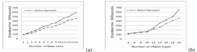
We evaluated the effect of the number of time slots on the execution time of the MDCOP algorithms using the real data set. The participation index, time prevalence index, and distance were set at 0.2, 0.8, and 100 m respectively. Experiments were run for a minimum of 1 time slot and a maximum of 14 time slots. Results show that the MDCOP Graph Miner requires less execution time than the fast MDCOP-Miner (Fig. 8a). As the number of time slots increases, the ratio of the increase in execution time is smaller for MDCOP Graph Miner than for the fast MDCOP-Miner. It shows that MDCOP Graph Miner has time cost advantage to fast MDCOP-Miner.
The participation index, time prevalence index, number of time slots, and distance were set at 0.2, 0.8,15, and 100 m, respectively. Results show that the MDCOP Graph Miner outperforms the fast MDCOP-Miner when the number of object-types increases (Fig. 8b). It is observed that the increase in execution time for the fast MDCOP-Miner is bigger than that of the MDCOP Graph Miner as the number of object-types increases for the real data set.
(a) (b)
Fig. 8. (a) Effect of number of time slots and object types using real data set
6.2. Experimental Results for Synthetic Datasets
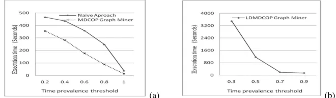
Effect of the Spatial Prevalence Threshold. We evaluated the effect of the spatial preva-lence threshold on the execution times of MDCOP mining algorithms. The fixed param-eters were time participation index, distance, and number of time slots, and their values were 0.8, 20 m, and 100, respectively. Experimental results show that the MDCOP Graph Miner this paper proposed is more computationally efficient than the fast MDCOP-Miner (Fig. 9a). The execution time of the MDCOP Graph Miner decreases as the spatial preva-lence threshold increases, and obviously MDCOP Graph Miner is running less time than fast MDCOP-Miner with all spatial prevalence.
We also evaluated the effect of the spatial prevalence threshold on the execution time of the LDMDCOP Graph Miner using synthetic data sets. The participation index, dis-tance and number of time slots, were set at 0.8, 20 m, 100, respectively. The results showed that the execution time of the LDMDCOP Graph Miner decreases as the time prevalence threshold increases (Fig. 9b).
(a) (b)
Fig. 9. (a), (b) Effect of the spatial prevalence threshold using synthetic data sets
were spatial participation index, distance, and number of time slots, and their values were 0.4, 20 m, and 100, respectively. Experimental results show that the MDCOP Graph Miner this paper proposed is more computationally efficient than the fast MDCOP-Miner (Fig. 10a). The execution time of the MDCOP Graph Miner decreases more than fast MDCOP-Miner as the spatial prevalence threshold increases.
We also evaluated the effect of the time prevalence threshold on the execution time of the LDMDCOP Graph Miner using synthetic data sets. The participation index, distance and number of time slots, were set at 0.5, 20 m, 100, respectively. The results showed that the execution time of the LDMDCOP Graph Miner decreases as the time prevalence threshold increases (Fig. 10b).
(a) (b)
Fig. 10.((a), (b) Effect of the time prevalence threshold using synthetic data sets
7.
Conclusions and Future Work
In the exception detection, there are many data attributes in the data packet captured in the network. There are a lot of useless and redundant attributes, As the dimension of data object increases, the cost of intrusion detection system increases exponentially. It will not only consume a large amount of storage space, but also greatly increase the time and space complexity of the intrusion detection program. Excessive dimensions will not only increase the resource consumption of the system, but also reduce the accuracy of detection.
method to improve calculation efficiency. In this paper, we presented a novel and com-putationally efficient algorithm (the MDCOP Graph Miner) for mining MDCOPs with large attack dataset. MDCOP Graph Miner represents the close relationship between the instances with MDCOP Graph structure; obtain information for mining co-occurrence patterns efficiently through accessing MDCOP Graph and design an effective pruning strategy simultaneously. Experiments show that MDCOP Graph Miner algorithm can not only get the complete and correct spatiotemporal co-occurrence patterns, but also improve computational efficiency.
Although MDCOP Graph Miner algorithm improves the efficiency in mixed-drove spatiotemporal co-occurrence patterns detection, but for large spatial and temporal attack data processing and analysis capabilities, or lack of. In order to solve this problem, on the basic of MDCOP Graph Miner, we presented an improved MDCOP Graph Miner algorithm (the LDMDCOP Graph Miner) which can deal with large spatiotemporal at-tack data sets. LDMDCOP Graph Miner takes MDCOP Graph as the storage structure for close relationships between instances, and storage MDCOP Graph on the hard disk. In the process of calculation, only the necessary attack data is loaded into memory, so as to solve attack data storage problems. Meanwhile, LDMDCOP Graph Miner makes index for MDCOP Graph, which improves the data query efficiency. Experiments show that LD-MDCOP Graph Miner algorithm can not only get the complete and correct mixed-drove spatiotemporal co-occurrence patterns detection, as well as have high computational effi-ciency.
In the future, we will extend the MDCOP graph and the subsequent mining algorithm for insertions of object attack types at arbitrary time interval. We hope to investigate the idea of multi-scale relationship for different co-occurrence patterns detection.
References
1. A.Garaeva, Makhmutova, F., Anikin, I., Sattler, K.: A framework for co-location patterns min-ing in big spatial data. In: Petersbur, S. (ed.) 2017 XX IEEE International Conference on Soft Computing and Measurements (SCM) (2017)
2. Cao, H., Mamoulis, N., W.Cheung, D.: Discovery of collocation episodes in spatiotemporal data. ICDM pp. 823–827 (2006)
3. Celik, M., Shekhar, S., Rogers, J.P., Shine, J.A.: Mixed-drove spatio-temporal co-occurence pattern mining. IEEE Trans. Knowledge and Data Eng. 20(10), 85–99 (2006)
4. D, Barbara0.and J, C., S, Jajodia.and N, W.: A testbed for exploring the use of data mining in intrusion detection acm sigmod record. Special section on data mining for intrusion detection and threat analysis (2001) pp. 15–24 (2001)
5. Ding, Z., Güting, R.H.: Modeling temporally variable transportation networks. DASFAA pp. 154–168 (2004)
6. Ekkehard, K., Katharina, L., Martin, S.: Time-expanded graphs for flow-dependent transit times. In: Algorithms—ESA 2002, Lecture Notes in Comput. Sci., vol. 2461, pp. 599–611. Springer, Berlin (2002)
7. George, B., Shekhar, S.: Time-aggregated graphs for modeling spatiotemporal networks. ER (Workshops) pp. 85–99 (2006)
9. Huang, Y., Shekhar, S., Xiong, H.: Discovering co-location patterns from spatial data sets: A general approach. IEEE Trans,Data Eng 16(12), 1472–1485 (2004)
10. J.Gudmundsson, V.Kreveld, M., Speckmann, B.: Efficient detection of motion patterns in spatio-temporal data sets. pp. 250–257. ACM-GIS (2004)
11. J.S.Yoo, Shekhar, S.: A partial join approach for mining co-location patterns. Proc. 12th Ann. ACM Int0l Workshop Geographic Information Systems (ACM-GIS) (2005)
12. J.S.Yoo, Shekhar, S., M.Celik: A join-less approach for co-location pattern mining: A summary of results. Proc. Fifth IEEE Int0l Conf. Data Mining (ICDM) (2005)
13. Kalnis, P., Mamoulis, N., Bakiras, S.: n discovering moving clusters in spatio-temporal data. 9th Int0l Symp. on Spatial and Temporal Database(SSTD) (2005)
14. Mete, C., Shashi, S., James, R., James, A.S., Jin, S.Y.: Mixed-drove spatio-temporal co-occurence pattern mining: A summary of results. Proceedings - IEEE International Conference on Data Mining, ICDM pp. 119–128 (12 2006)
15. Minwei, T., Zhanquan, W.: Research of spatial co-location pattern mining based on segmenta-tion threshold weight for big dataset. ICSDM 2015 - Proceedings 2015 2nd IEEE Internasegmenta-tional Conference on Spatial Data Mining and Geographical Knowledge Services pp. 49–54 (2015) 16. S.Banerjee, Carlin, B., Gelfrand, A.: Hierarchical modeling and analysis for spatial data. CRC
Press 22(2), 115–170 (2003)
17. Shekhar, S., Huang, Y.: Discovering spatial co-location patterns: A summary of results (2001) 18. S.Shekhar, Huang, Y., Xiong, H.: Discovering spatial co-location patterns: A summary of
re-sults. pp. 236–256. Proc. Seventh Int0l Symp. Spatial and Temporal Databases (SSTD 001) (2001)
19. Tsang, C.H., Kwong, S., Wang, H.: Genetic-fuzzy rule mining approach and evaluation of feature selection techniques for anomaly intrusion detection. Pattern Recognition 40(9), 2373 – 2391 (2007)
20. Y, H., S, S., H, X.: Discovering co-location patterns from spatial datasets: a general approach. IEEE Transactions on Knowledge and Data Engineering (TKDE) 16(12), 1472–1485 (2004)
Zhanquan Wangis an associate professor at Department of Computer Science and En-gineering of East China University of Science and Technology in Shanghai, China. He received his Ph.D. in computer science from Zhejiang University in China in 2005. His current research interests include Spatial Datamining, GIS, Educational technology. Con-tact him at [email protected].
Taoli Hanis currently a Master candidate at East China University of Science and Tech-nology in Shanghai, China. He received his bachelor’s degree in Computer science and technology from Hainan University in Haikou, China in 2017. Her current research inter-ests include datamining, spatial datamining. Contact him at [email protected].
Huiqun Yu(Corresponding Author) is professor and PhD supervisor, received the PhD degree from the department of computer science, ShangHai JiaoTong University, in 1995. He is the senior member of IEEE and China Computer Federation and ACM members. His main research interests include trusted computing, cloud computing, software engineering and service oriented software in cloud. Contact him at [email protected]