Deep Learning-An Upcoming Technology

RESEARCH ARTICLE

DEEP LEARNING-AN UPCOMING TECHNOLOGY

1

_{Krupa, T. K. and}

_{Venkatagiri, J.}

1

_{Assistant Professor, Computer Science and Engineering, Sri Venkateshwara College of Engineering, Bangalore,}

Karnataka, India

2

_{UG Student, Computer Science and Engineering, Sri Venkateshwara College of Engineering}

_,

_Bangalore,

Karnataka, India

ARTICLE INFO

ABSTRACT

Deep learning allows computational models that are composed of multiple processing layers to learn representations of data with multiple levels of abstraction. These methods have dramatically improved the state-of-the-art in speech recognition, visual object recognition, object detection and many other domains such as drug discovery and genomics. Deep learning discovers intricate structure in large data sets by using the backpropagation algorithm to indicate how a machine should change its internal parameters that are used to compute the representation in each layer from the representation in the previous layer. Deep convolutional nets have brought about breakthroughs in processing images, video, speech and audio, whereas recurrent nets have shone light on sequential data such as text and speech.

Copyright©2017,Krupa and Venkatagiri. This is an open access article distributed under the Creative Commons Attribution License, which permits unrestricted

use, distribution, and reproduction in any medium, provided the original work is properly cited.

INTRODUCTION

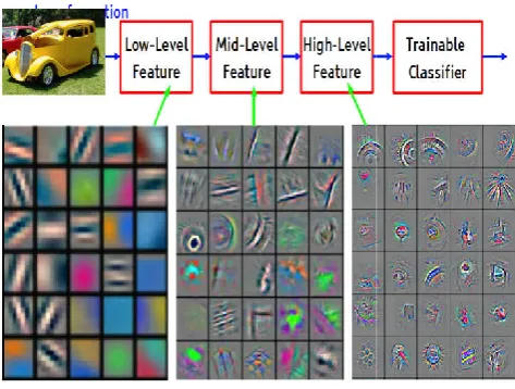
Machine-learning technology powers many aspects of modern society: from web searches to content filtering on social networks to recommendations on e-commerce websites, and it is increasingly present in consumer products such as cameras and smartphones. Machine-learning systems are used to identify objects in images, transcribe speech into text, match news items, posts or products with users’ interests, and select relevant results of search. Increasingly, these applications make use of a class of techniques called deep learning. Conventional machine-learning techniques were limited in their ability to process natural data in their raw form. For decades, constructing a pattern-recognition or machine-learning system required careful engineering and considerable domain expertise to design a feature extractor that transformed the raw data (such as the pixel values of an image) into a suitable internal representation or feature vector from which the learning subsystem, often a classifier, could detect or classify patterns in the input. Representation learning is a set of methods that allows a machine to be fed with raw data and to automatically discover the representations needed for detection or classification.

*Corresponding author: Krupa, T. K.,

Assistant Professor, Computer Science and Engineering, Sri Venkateshwara College of Engineering, Bangalore, Karnataka, India

Deep-learning methods are representation-learning methods with multiple levels of representation, obtained by composing simple but non-linear modules that each transform the representation at one level (starting with the raw input) into a representation at a higher, slightly more abstract level.

Supervised Learning

The most common form of machine learning, deep or not, is supervised learning. Imagine that we want to build a system that can classify images as containing, say, a house, a car, a person or a pet. We first collect a large data set of images of houses, cars, people and pets, each labelled with its category. During training, the machine is shown an image and produces an output in the form of a vector of scores, one for each category. We want the desired category to have the highest score of all categories, but this is unlikely to happen before training. We compute an objective function that measures the error (or distance) between the output scores and the desired pattern of scores. The machine then modifies its internal adjustable parameters to reduce this error. These adjustable parameters, often called weights, are real numbers that can be seen as ‘knobs’ that define the input–output function of the machine. In a typical deep-learning system, there may be hundreds of millions of these adjustable weights, and hundreds of millions of labelled examples with which to train the

ISSN: 0976-3376

Available Online at http://www.journalajst.com

ASIAN JOURNAL OF

SCIENCE AND TECHNOLOGY

Article History:

Received 22nd _{June, 2017}

Received in revised form 28th _{July, 2017}

Accepted 06th _{August, 2017}

Published online 27th _{September, 2017}

Key words:

Machine. To properly adjust the weight vector, the learning algorithm computes a gradient vector that, for each weight, indicates by what amount the error would increase or decrease if the weight were increased by a tiny amount. The weight vector is then adjusted in the opposite direction to the gradient vector. The objective function, averaged over all the training examples, can be seen as a kind of hilly landscape in the high dimensional space of weight values.

Fig. 1. Deep learning representation

The negative gradient vector indicates the direction of steepest descent in this landscape, taking it closer to a minimum, where the output error is low on average. In practice, most practitioners use a procedure called stochastic gradient descent (SGD). This consists of showing the input vector for a few examples, computing the outputs and the errors, computing the average gradient for those examples, and adjusting the weights accordingly. The process is repeated for many small sets of examples from the training set until the average of the objective function stops decreasing. It is called stochastic because each small set of examples gives a noisy estimate of the average gradient over all examples. This simple procedure usually finds a good set of weights surprisingly quickly when compared with far more elaborate optimization techniques18. After training, the performance of the system is measured on a different set of examples called a test set.

Fig. 2. Deep learning a breakthrough technology

. To properly adjust the weight vector, the learning algorithm computes a gradient vector that, for each weight, indicates by what amount the error would increase or decrease weight were increased by a tiny amount. The weight vector is then adjusted in the opposite direction to the gradient vector. The objective function, averaged over all the training examples, can be seen as a kind of hilly landscape in the

high-Fig. 1. Deep learning representation

The negative gradient vector indicates the direction of steepest descent in this landscape, taking it closer to a minimum, where the output error is low on average. In practice, most ioners use a procedure called stochastic gradient descent (SGD). This consists of showing the input vector for a few examples, computing the outputs and the errors, computing the average gradient for those examples, and adjusting the weights he process is repeated for many small sets of examples from the training set until the average of the objective function stops decreasing. It is called stochastic because each small set of examples gives a noisy estimate of amples. This simple procedure usually finds a good set of weights surprisingly quickly when compared with far more elaborate optimization techniques18. After training, the performance of the system is measured on a

rning a breakthrough technology

This serves to test the generalization ability of the machine its ability to produce sensible answers on new inputs that it has never seen during training.

Back propagation to train multilayer

From the earliest days of pattern recognition22, 23, the aim of researchers has been to replace hand

trainable multilayer networks, but despite its simplicity, the solution was not widely understood until the

turns out, multilayer architectures can be trained by simp stochastic gradient descent.

relatively smooth functions of their inputs and of their internal weights, one can compute gradients using the backpropaga procedure. The idea that this could be done, and that it worked, was discovered independently by several different groups during the 1970s and 1980s2

procedure to compute the gradient of an objective function with respect to the weights of a multilayer stack of modules is nothing more than a practical application of the chain Rule for derivatives. The key insight is that the derivative (or gradient) of the objective with respect to the input of a module can be computed by working backwards from the gradient with respect to the output of that module (or the input of the subsequent module). The back

applied repeatedly to propagate gradients through all modules, starting from the output at the top (where

produces its prediction) all the way to the bottom (where the external input is fed). Once these gradients have been computed, it is straightforward to compute the gradients with respect to the weights of each module. Many applications of deep learning use feed forward neural network architectures, which learn to map a fixed-size input (for example, an image) to a fixed-size output (for example, a probability for each of several categories). To go from one layer to the next, a set of units compute a weighted sum of their inputs from the previous layer and pass the result through a non function. At present, the most popular non

the rectified linear unit (ReLU), which is simply the half rectifier f (z) = max (z, 0). In past decades, neural nets used smoother non-linearities, such as tanh(z) or 1/(1 + exp( but the ReLU typically learns much faster in networks with many layers, allowing training of a deep supervised network without unsupervised pre-training28. Unit

input or output layer are conventionally called hidden units.

The hidden layers can be seen as distorting the input in a non linear way so that categories become linearly separable by the last layer. In the late 1990s, neural nets an

were largely forsaken by the machine

ignored by the computer-vision and speech

communities. It was widely thought that learning useful, multistage, feature extractors with little prior knowledge was infeasible. In particular, it was commonly thought that simple gradient descent would get trapped in poor local minima weight configurations for which no small change would reduce the average error. In practice, poor local minima are rarely a problem with large networks. Regardless of the initial conditions, the system nearly always reaches solutions of very similar quality. Recent theoretical and empirical results strongly suggest that local minima are not a serious issue in

general. Instead, the landscape i

combinatorially large number of saddle points where the gradient is zero, and the surface curves up in most dimensions This serves to test the generalization ability of the machine — its ability to produce sensible answers on new inputs that it has

Back propagation to train multilayer architectures

From the earliest days of pattern recognition22, 23, the aim of researchers has been to replace hand-engineered features with trainable multilayer networks, but despite its simplicity, the solution was not widely understood until the mid-1980s. As it turns out, multilayer architectures can be trained by simple stochastic gradient descent. As long as the modules are relatively smooth functions of their inputs and of their internal weights, one can compute gradients using the backpropagation procedure. The idea that this could be done, and that it worked, was discovered independently by several different groups during the 1970s and 1980s24–27. The backpropagation procedure to compute the gradient of an objective function he weights of a multilayer stack of modules is nothing more than a practical application of the chain Rule for derivatives. The key insight is that the derivative (or gradient) of the objective with respect to the input of a module can be ng backwards from the gradient with respect to the output of that module (or the input of the subsequent module). The back propagation equation can be applied repeatedly to propagate gradients through all modules, starting from the output at the top (where the network produces its prediction) all the way to the bottom (where the external input is fed). Once these gradients have been computed, it is straightforward to compute the gradients with respect to the weights of each module. Many applications of forward neural network architectures, size input (for example, an image) size output (for example, a probability for each of several categories). To go from one layer to the next, a set of ute a weighted sum of their inputs from the previous layer and pass the result through a non-linear function. At present, the most popular non-linear function is the rectified linear unit (ReLU), which is simply the half-wave In past decades, neural nets used linearities, such as tanh(z) or 1/(1 + exp(−z)), but the ReLU typically learns much faster in networks with many layers, allowing training of a deep supervised network training28. Units that are not in the input or output layer are conventionally called hidden units.

The hidden layers can be seen as distorting the input in a non-linear way so that categories become non-linearly separable by the last layer. In the late 1990s, neural nets and backpropagation were largely forsaken by the machine-learning community and vision and speech-recognition communities. It was widely thought that learning useful, multistage, feature extractors with little prior knowledge was asible. In particular, it was commonly thought that simple gradient descent would get trapped in poor local minima — weight configurations for which no small change would reduce the average error. In practice, poor local minima are rarely a rge networks. Regardless of the initial conditions, the system nearly always reaches solutions of very similar quality. Recent theoretical and empirical results strongly suggest that local minima are not a serious issue in

general. Instead, the landscape is packed with a

and curves down in the remainder29, 30. The analysis seems to show that saddle points with only a few downward curving directions are present in very large numbers, but almost all of them have very similar values of the objective function. Hence, it does not much matter which of these saddle points the algorithm gets stuck at. Interest in deep feedforward networks was revived around 2006 by a group of researchers brought together by the Canadian Institute for Advanced Research (CIFAR).

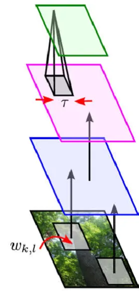
Fig. 3. Layers, inputs and outputs processing in deep learning layers

Convolutional neural Networks

ConvNets are designed to process data that come in the form of multiple arrays, for example a colour image composed of three 2D arrays containing pixel intensities in the three colour channels. Many data modalities are in the form of multiple arrays: 1D for signals and sequences, including language; 2D for images or audio spectrograms; and 3D for video or volumetric images. There are four key ideas behind ConvNets that take advantage of the properties of natural signals: local connections, shared weights, pooling and the use of many layers. The architecture of a typical ConvNet is structured as a series of stages. The first few stages are composed of two types of layers: convolutional layers and pooling layers. Units in a convolutional layer are organized in feature maps, within which each unit is connected to local patches in the feature maps of the previous layer through a set of weights called a filter bank. The result of this local weighted sum is then passed through a non-linearity such as a ReLU. All units in a feature map share the same filter bank. Different feature maps in a layer use different filter banks. The reason for This architecture is twofold. First, in array data such as images, local groups of values are often highly correlated, forming distinctive local motifs that are easily detected. Second, the local statistics of images and other signals are invariant to location. In other words, if a motif can appear in one part of the image, it could appear anywhere, hence the idea of units at different locations sharing the same weights and detecting the same pattern in different parts of the array. Mathematically, the filtering operation performed by a feature map is a discrete convolution, hence the name. Although the role of the convolutional layer is to detect local conjunctions of features from the previous layer, the role of the pooling layer is to merge semantically similar features into one. Because the relative positions of the features forming a motif can vary somewhat, reliably detecting the motif can be done by coarse-graining the position of each feature. A typical pooling unit computes the maximum of a local patch of units in one feature map (or in a few feature maps). Neighboring pooling units take input from patches that are shifted by more than one row or column, thereby reducing the dimension of the representation and creating an invariance to small shifts and distortions.

Fig. 4. Convolutional neural networks

Image understanding with deep convolutional networks

Since the early 2000s, ConvNets have been applied with great success to the detection, segmentation and recognition of objects and regions in images. These were all tasks in which labelled data was relatively abundant, such as traffic sign recognition, the segmentation of biological images particularly for connectomics, and the detection of faces, text, pedestrians and human bodies in natural images. A major recent practical success of ConvNets is face recognition. Importantly, images can be labelled at the pixel level, which will have applications in technology, including autonomous mobile robots and self-driving cars. Companies such as Mobileye and NVIDIA are using such ConvNet-based methods in their upcoming vision systems for cars. Other applications gaining importance involve natural language understanding14 and speech recognition7. Despite these successes, ConvNets were largely forsaken by the mainstream computer-vision and machine-learning communities until the Image Net competition in 2012. When deep convolutional networks were applied to a data set of about a million images from the web that contained 1,000 different classes, they achieved spectacular results, almost halving the error rates of the best competing approaches1. This success came from the efficient use of GPUs, ReLUs, a new regularization technique called dropout62, and techniques to generate more training examples by deforming the existing ones. This success has brought about a revolution in computer vision; ConvNets are now the dominant approach for almost all recognition and detection tasks4 and approach human performance on some tasks. A recent stunning demonstration combines ConvNets and recurrent net modules for the generation of image captions Recent ConvNet architectures have 10 to 20 layers of ReLUs, hundreds of millions of weights, and billions of connections between units. Whereas training such large networks could have taken weeks only two

years ago, progress in hardware, software and algorithm parallelization have reduced training times to a few hours. The performance of ConvNet-based vision systems has caused most major technology companies, including Google, Facebook, Microsoft, IBM, Yahoo!, Twitter and Adobe, as well as a quickly growing number of start-ups to initiate research and development projects and to deploy ConvNet-based image understanding products and services. ConvNets are easily amenable to efficient hardware implementations in chips or field-programmable gate arrays. A number of companies such as NVIDIA, Mobileye, Intel, Qualcomm and Samsung are developing ConvNet chips to enable real-time vision applications in smartphones, cameras, robots and self-driving cars.

Distributed representations and language processing

Deep-learning theory shows that deep nets have two different exponential advantages over classic learning algorithms that do not use distributed representations21. Both of these advantages arise from the power of composition and depend on the underlying data-generating distribution having an

appropriate componential structure40. First, learning

distributed representations enable generalization to new combinations of the values of learned features beyond those seen during training (for example, 2n combinations are possible with n binary features) 68, 69. Second, composing layers of representation in a deep net brings the potential for another exponential advantage70 (exponential in the depth). The hidden layers of a multilayer neural network learn to represent the network’s inputs in a way that makes it easy to predict the target outputs. This is nicely demonstrated by training a multilayer neural network to predict the next word in a sequence from a local context of earlier words71. Each word in the context is presented to the network as a one-of-N vector, that is, one component has a value of 1 and the rest are 0. In the first layer, each word creates a different pattern of activations, or word vectors (Fig. 4). In a language model, the other layers of the network learn to convert the input word vectors into an output word vector for the predicted next word, which can be used to predict the probability for any word in the vocabulary to appear as the next word. The network learns word vectors that contain many active components each of which can be interpreted as a separate feature of the word, as was first demonstrated27 in the context of learning distributed representations for symbols. These semantic features were not explicitly present in the input.

They were discovered by the learning procedure as a good way of factorizing the structured relationships between the input and output symbols into multiple ‘micro-rules’. Learning word vectors turned out to also work very well when the word sequences come from a large corpus of real text and the individual micro-rules are unreliable71. When trained to predict the next word in a news story, for example, the learned word vectors for Tuesday and Wednesday are very similar, as are the word vectors for Sweden and Norway. Such representations are called distributed representations because their elements (the features) are not mutually exclusive and their many configurations correspond to the variations seen in the observed data. These word vectors are composed of learned features that were not determined ahead of time by experts, but automatically discovered by the neural network. Vector representations of words learned from text are now

very widely used in natural language applications. The issue of representation lies at the heart of the debate between the logic-inspired and the neural-network-logic-inspired paradigms for cognition. In the logic-inspired paradigm, an instance of a symbol is something for which the only property is that it is either identical or non-identical to other symbol instances. It has no internal structure that is relevant to its use; and to reason with symbols, they must be bound to the variables in judiciously chosen rules of inference. By contrast, neural networks just use big activity vectors, big weight matrices and scalar non-linearities to perform the type of fast ‘intuitive’ inference that underpins effortless commonsense reasoning. Before the introduction of neural language models71, the standard approach to statistical modelling of language did not exploit distributed representations: it was based on counting frequencies of occurrences of short symbol sequences of length up to N (called grams). The number of possible N-grams is on the order of VN, where V is the vocabulary size, so taking into account a context of more than a handful of work.

Recurrent Neural Networks

the meaning of an image into an English sentence. The encoder here is a deep ConvNet that converts the pixels into an activity vector in its last hidden layer. The decoder is an RNN similar to the ones used for machine translation and neural language modelling. There has been a surge of interest in such systems recently (see examples mentioned in ref.). RNNs, once unfolded in time, can be seen as very deep feedforward networks in which all the layers share the same weights.

Future of deep learning

Unsupervised learning had a catalytic effect in reviving interest in deep learning, but has since been overshadowed by the successes of purely supervised learning. Although we have not focused on it in this Review, we expect unsupervised learning to become far more important in the longer term. Human and animal learning is largely unsupervised: we discover the structure of the world by observing it, not by being told the name of every object. Human vision is an active process that sequentially samples the optic array in an intelligent, task-specific way using a small, high-resolution fovea with a large, low-resolution surround. We expect much of the future progress in vision to come from systems that are trained end-toend and combine ConvNets with RNNs that use reinforcement learning to decide where to look. Systems combining deep learning and reinforcement learning are in their infancy, but they already outperform passive vision systems99 at classification tasks and produce impressive results in learning to play many different video games. Natural language understanding is another area in which deep learning is poised to make a large impact over the next few years. We expect systems that use RNNs to understand sentences or whole documents will become much better when they learn strategies for selectively attending to one part at a time. Ultimately, major progress in artificial intelligence will come about through systems that combine representation learning with complex reasoning. Although deep learning and simple reasoning have been used for speech and handwriting recognition for a long time, new paradigms are needed to replace rule-based manipulation of symbolic expressions by operations on large vectors.

Conclusion

Deep learning = Learning Hierarchical Representations

Deep learning is thriving in big data analytics, including image

processing, speech recognition, and natural language

processing.

Deep learning has matured and is very promising as an artificial intelligence method.

Still has room for improvement: Scaling computation

Optimization

Bypass intractable marginalization More disentangled abstractions

Reasoning from incrementally added facts.

REFERENCES

Farabet, C., Couprie, C., Najman, L. and LeCun, Y. 2013. Learning hierarchical features for scene labeling. IEEE Trans. Pattern Anal. Mach. Intell. 35, 1915–1929.

Hinton, G. et al. 2012. Deep neural networks for acoustic modeling in speech recognition. IEEE Signal Processing Magazine 29, 82–97. This joint paper from the major

speech recognition laboratories, summarizing the

breakthrough achieved with deep learning on the task of phonetic classification for automatic speech recognition, was the first major industrial application of deep learning. Krizhevsky, A., Sutskever, I. and Hinton, G. 2012. ImageNet

classification with deep convolutional neural networks. In Proc. Advances in Neural Information Processing Systems 25 1090–1098. This report was a breakthrough that used convolutional nets to almost halve the error rate for object recognition, and precipitated the rapid adoption of deep learning by the computer vision community.

Mikolov, T., Deoras, A., Povey, D., Burget, L. and Cernocky, J. 2011. Strategies for training large scale neural network language models. In Proc. Automatic Speech Recognition and Understanding 196–201.

Szegedy, C. et al. 2014. Going deeper with convolutions. Preprint at http://arxiv.org/ abs/1409.4842.

Tompson, J., Jain, A., LeCun, Y. and Bregler, C. 2014. Joint training of a convolutional network and a graphical model

for human pose estimation. In Proc. Advances in Neural

Information Processing Systems 27 1799–1807.

*******