Online Clustering for Trajectory Data Stream of
Moving Objects
Yanwei Yu1,2, Qin Wang1,2, Xiaodong Wang1, Huan Wang1, and Jie He1
1 School of Computer and Communication Engineering,
University of Science and Technology Beijing 100083 Beijing, China
2 Beijing Key Laboratory of Knowledge Engineering for Materials Science
100083 Beijing, China [email protected]
Abstract. Trajectory data streams contain huge amounts of data pertain-ing to the time and position of movpertain-ing objects. It is crucial to extract use-ful information from this peculiar kind of data in many application sce-narios, such as vehicle traffic management, large-scale tracking manage-ment and video surveillance. This paper proposes a density-based clus-tering algorithm for trajectory data stream called CTraStream. It contains two stages: trajectory line segment stream clustering and online trajec-tory cluster updating. CTraStream handles the trajectrajec-tory data of moving objects as an incremental line segment stream. For line segment stream clustering, we present a distance measurement approach between line segments. Incremental line segments are processed quickly based on previous line clusters in order to achieve clustering line segment stream online, and line-segment-clusters in a time interval are obtained on the fly. For online trajectory cluster updating, TC-Tree, an index structure, which stores all closed trajectory clusters, is designed. According to the line-segment-cluster set, the current closed trajectory clusters are updated online based on TC-Tree by performing proposed update rules. The algo-rithm has exhibited many advantages, such as high scalability to process incremental trajectory data streams and the ability to discover trajectory clusters in data streams in real time. Our performance evaluation exper-iments conducted on a number of real and synthetic trajectory datasets illustrate the effectiveness, efficiency, and scalability of the algorithm.
Keywords:trajectory stream clustering, density-based clustering, line seg-ment cluster, trajectory cluster, TC-Tree, online.
1.
Introduction
to extract useful information in the trajectory streams has become very impor-tant. Therefore, incremental trajectory data stream mining is receiving a lot of attentions. Trajectory clustering, which groups the trajectories of moving objects to reveal interesting correlations among them, has a number of applications in vehicle traffic management, logistics management, pattern recognition, and be-havior analysis [21]. For example, clustering the trajectory data stream of mov-ing objects in real time can obtain some motion patterns to help administrators to predict movement trends and prevent anomalous events from occurring in a large security system. Density-based clustering can discover the clusters with arbitrary shapes and filter out noise, which is very useful for identifying the rela-tions of moving objects whose mobile direction is stochastic and unpredictable. Thus, an efficient clustering algorithm based on density is essential for trajec-tory data streams analysis in these applications with real time constraint.
In this paper, regarding to clustering trajectory data streams that pertain to time and the position of moving objects, we propose a clustering algorithm, CTraStream, which can discover the trajectory clusters with explicit temporal information and spatial information from data streams. The following contribu-tions are made: First, we provide a definition of distance measure between trajectory line segments, and, by employing the distance measure, CTraStream performs density-based clustering on received trajectory line segment streams to obtain line segment clusters in real time. Second, a TC-Tree structure is designed, which stores the closed trajectory clusters and represents the rela-tionship among trajectory clusters. Finally, the trajectory clusters on TC-Tree is updated according to the line segment clusters online. Comprehensive empir-ical studies on real data and large synthetic data demonstrate the clustering effectiveness, efficiency, and scalability of our developed algorithm.
The remainder of this paper is organized as follows: We discuss related clus-tering algorithms in Section 2. In Section 3, we first define the basic notions of our algorithm and introduce the general framework of CTraStream. A detailed description of CLnStream, a density-based line segment stream clustering al-gorithm, is provided in Section 4, and TraCluUpdate, a online update process of trajectory cluster, is presented in Section 5. Evaluation experiments of ef-fectiveness and efficiency are shown in Section 6. Finally, Section 7 presents conclusions and points out directions for future work.
2.
Related Works
using the maximum likelihood principle. Specially, the EM algorithm is used to estimate hidden parameters involved in probability models, and then deter-mine the clusters membership. But the basic processing unit of the clustering is the whole trajectory. Nanni [15] adapts two classical distance-based clustering methods (K-means and hierarchical agglomerative clustering) to trajectories. Then, Nanni et al [19] propose a time-focused trajectory clustering algorithm based on density. In Their paper, a simple notion of distance between trajecto-ries is first defined, and then a new approach to trajectory clustering problems based on OPTICS, called temporal focusing, is presented, which aims to ex-ploit the intrinsic semantics of temporal dimensions to improve the quality of trajectory clustering.
Piciarelli et al. [2] propose a trajectory clustering algorithm suited for on-line behavior analysis. The incremental trajectories are matched with previous clusters in space and grouped into the closest clusters, and the clusters are or-ganized in a tree-like structure, which can be used to detect anomalous events. Lee et al. [8] present a trajectory clustering framework based on density, called TRACLUS, which is a partition-and-group framework for discovering common sub-trajectories in trajectory databases. In the partition phase, trajectories are partitioned into a set of quasi-linear segments using the minimum description length principle. In the group phase, all line segments are grouped using a density-based clustering method, and a representative trajectory for each clus-ter is declus-termined. Based on TRACLUS, Lee et al. [9] succeedingly propose a feature generation framework TraClass for trajectory classification. It generates a hierarchy of features by partitioning trajectories and exploring region-based and trajectory-based clustering. Zhenhui Li et al. [27] propose a clustering framework for incremental trajectory called TCMM, which contains online micro-cluster maintenance and offline macro-micro-cluster creation. The former is used to incrementally update the micro-clusters that store compact summaries of sim-ilar line segments to reflect the changes; the latter performs macro-clustering based on the set of micro-clusters when a user requests to see current clus-tering result. All of TRACLUS, TraClass and TCMM employ the density-based clustering method, but trajectories are represented as sequences of line seg-ments without explicit temporal information.
min-imal bounding boxes (MBBs), and a similarity between two trajectories based on MBBs is defined. With the definition, the method employs a trajectory-fitted version of the incremental K-mean algorithm for clustering moving objects. With similar objective, Jensen et al. [3] present a scheme that is capable of incre-mentally clustering moving objects. It employs a notion of object dissimilarity and clustering features, and uses a quality measure for incremental clusters to identify clusters that are not compact enough after certain insertions and dele-tions. Although the objectives of such algorithms are a somewhat different, they focus on the efficient discovery of static clusters at variable time snapshots.
Won et al [12] propose a trajectory clustering scheme for vehicles moving on road networks, which defines a trajectory as a sequence of road segments a moving object has passed by. The scheme modifies and adjusts FastMap and hierarchical clusters by measuring total length of matched road segments, and yields fairly accurate clustering results. However, the algorithm only can work on clustering objects in a spatial network. Kalnis et al. [13] provide a for-mal definition of moving clusters to discover a set of objects that move close to each other for a long time interval. During the time interval, some objects may leave or enter the cluster, but the portion of common objects should be higher than a predefined threshold in two continuous timestamps. Jeung et al. [10] define a convoy pattern, in which a set of objects that move together in a cluster with arbitrary shapes during at least k continuous timestamps. They propose three algorithms involving trajectory simplification techniques to query the convoy patterns from trajectory databases in a filter-refinement framework. However, these works cannot handle trajectory data streams efficiently since clusters are re-calculated from scratch every time. Efficient maintenance of such meta-trajectory clusters on streams requires a thorough analysis of the spatio-temporal properties of moving objects, which is a key issue addressed in our work.
3.
Problem Formulation
3.1. Notion Definition
Trajectory data stream in which there areN moving objects is defined as fol-lows:S=(P0
1P20. . . Pi0. . . Pn0P11P21. . . Pi1. . . Pn1. . . P j 1P
j 2. . . P
j
i . . . Pnj. . . P1kP2k. . . Pik. . . Pnk. . .). Where,P
j
i is location of thei
thmoving object at the jth times-tamp. Real time positions of moving objects at each sampling time interval are received in form of data stream.
Definition 1.(Trajectory line segment) For moving objectO, its position is
pi when timestamp is ti, and position is pi+1 when timestamp istt+1. Vector −−−−→
pipi+1is called a trajectory line segment of the moving objectO, also known as line segment.
Definition 2.(Line segments distance) For line segments of two moving objects during same time interval, the distance between li and lj is defined as formula (1), which is composed of three components: start distance, center distance, and end distance.
dist(li, lj) =α∗dstart(li, lj) +β∗dcenter(li, lj) +γ∗dend(li, lj) (1)
dstart(li, lj) =|ps
i −psj|is the distance betweenpsi the starting point of seg-ment li and psj the starting point of segment lj, dcenter(li, lj) = |a−b| is the distance between athe midpoint of the segmentli andb the midpoint of the segmentlj,dend(li, lj) =|pei −pej|is the distance betweenpei the end point ofli andpejthe end point oflj.α, β, γ, respectively, stands for the weight of the start distance, the center distance and end distance.
Fig. 1.Distance between line segments.θis the included angle ofliandlj.
The weights are relative toθthe included angle of the two line segments, as defined in formula (2).
α= (1−sinθ/2)/3
β= 1/3
γ= (1 +sinθ/2)/3
,0≤θ≤π/2
α= (sinθ/2)/3
β = 1/3
γ= (2−sinθ/2)/3
, π/2< θ≤π
(2)
By formula (2), when the included angleθ is zero, the start distance, the center distance, and the end distance occupy the same proportion; while the weight of end distance increases in the distance formula as angleθincreases.
Definition 3.(Neighborhood) For line segments li, the set {l|l ∈ D and dist(l, li)≤e}is called the neighborhood of segmentli, denoted byN LnsD(li), and let|N LnsD(li)|denotes the number ofN LnsD(li).
Definition 4.(Core line segment) A line segmentliis a core line segment if
|N LnsD(li)|is not less thanM inLns.
Definition 5.(Border line segment) If|N LnsD(li)|is less thanM inLns, but there is a core line segmentljsatisfyinglj ∈N LnsD(li), then the line segment liis called a border line segment of the line segment cluster containinglj.
Definition 6. (Isolated line segment) A line segmentli is an isolated line
segment only if it is neither a core line segment nor a border line segment.
Definition 7.(Directly density-reachable) If a line segment li is the
neigh-borhood of a core line segment lj, then li is directly density-reachable from lj.
Obviously,li is not necessarily a core line segment, solj is not necessarily directly density-reachable fromli, therefore, directly density-reachable is asym-metrical.
Definition 8. (Density-reachable) A line segment li is density-reachable
from a line segmentlj, if there is a series of line segmentsli, li+1, . . . , lj−1, lj ∈ Dsuch thatlk directly density-reachable fromlk+1(k=i, i+ 1, . . . , j−1, j).
Like directly density-reachable, density-reachable is also asymmetrical, but the density-reachable is transitive. Ifliis density-reachable from a line segment l, andlis density -reachable from a line segmentlj, thenliis density-reachable fromlj.
Definition 9.(Density-connected) If a line segmentli and a line segmentlj
are both density-reachable from a line segmentl, thenli is density-connected tolj.
According to the definition 9, density-connected is symmetrical for a pair of line segments.
Definition 10.(Line-segment-cluster) Grouping the setDinto a series of
in-dependent subset in which all line segments is density-connected to each other, each non-empty subsetCis called a line-segment-cluster, abbr. l-s-cluster, if it satisfies the following two conditions:
(1) Connectivity:∀li;lj∈C,liis density-connected tolj;
(2) Maximality:∀li;lj ∈D, ifli∈Candljis density-reachable fromli, then lj∈C.
Each l-s-cluster can be comprised of at least one core line segment and all line segments being density-reachable from one of the core line segments. The set of line-segment-clusters in time interval[i, i+ 1]is denoted asLC[i,i+1] = {lc1[i,i+1], lc2[i,i+1], . . . lck[i,i+1]}.
Lemma 1.A core line segment must and only belongs to a l-s-cluster.
Proof: LetDbe the current line segment set, and assume the core segment l belongs to two l-s-clusterslc1
[i,i+1], lc 2
[i,i+1]. Since the core line segment l ∈ lc1
[i,i+1], according to the definition of l-s-cluster, any line segmentl′belonging to lc1
l, therefore, any line segmentl′(l′ ∈lc1
[i,i+1])is density-reachable froml. Sim-ilarly, for any line segmentl′′(l′′ ∈lc2
[i,i+1])is also density-reachable from l. In conclusion, any line segmentl′(l′∈lc1
[i,i+1])andl′′(l′′∈lc 2
[i,i+1])are all density-connected to each other,lc1
[i,i+1], lc 2
[i,i+1]are the same l-s-cluster according to
the definition of l-s-cluster.
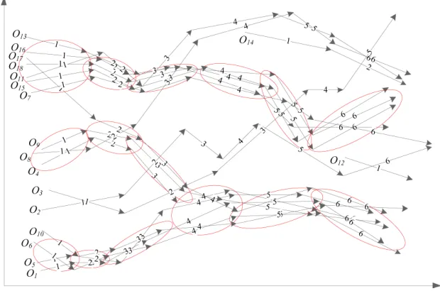
As shown in Fig. 2, there are 18 moving objects. Each line segment with an arrow stand for a trajectory line segment of the moving object, and the number marked on the line segment indicates the time interval of the line segment. Sup-posedM inLnsis 2, all line segments in a red ellipse constitute a line cluster.
Definition 11. (Trajectory cluster) For all moving objects in the trajectory
streamN, a 2-tuples(O,[i, j])is called a trajectory cluster if there existslcik
[k,k+1]∈ LC[k,k+1](k=i, i+1, . . . , j−1)such that the setO⊆
∩j−1 k=ilc
ik
[k,k+1](O∈N) dur-ing the time interval[i, j](j > i).Ois the set of objects in the trajectory cluster, andiandjis the start time and end time of the trajectory cluster respectively.
If(O,[i, j])is a trajectory cluster, and any 2-tuples(O′,[i, j]) (O′⊃O)is not a trajectory cluster, then(O,[i, j])is object-closed.
Fig. 2.An example of line segment clusters and trajectory clusters. Each line
segment with an arrow represents a trajectory line segment of the moving ob-ject, and the number on the line segment indicates the time interval of the line segment.
Lemma 2.For a set O(O ∈ N)including any m moving objects, if there
existslcik
[k,k+1] ∈LC[k,k+1](k =i, i+ 1, . . . , j−1) such thatO = ∩j−1
k=ilc ik
during time interval [i, j](j > i), then the 2-tuples(O,[i, j])is a object-closed trajectory cluster.
The lemma 2 is intuitive. SinceO=∩jk=i−1lcik
[k,k+1], for anyO′(O′ ⊃O),O′⊃ ∩j−1
k=ilc ik
[k,k+1],so the 2-tuples(O′,[i, j])is not a trajectory cluster by the defini-tion 11. Therefore, lemma 2 is proved.
If a 2-tuples(O,[i, j])is a trajectory cluster, and(O,[i−1, i])and(O,[j, j+1])
are not trajectory clusters, then(O,[i, j])is time-closed.
A trajectory cluster(O,[i, j])is called a closed trajectory cluster, if and only if (O,[i, j]) is both object-closed and time-closed. As shown in Fig. 2, the l-s-clusters of continuous time intervals constitute a closed trajectory cluster.
3.2. General Framework of CTraStream
CTraStream is divided into two online processes: line segment stream cluster-ing, CLnStream, which clusters the line segment stream of moving objects on-line to obtain the l-s-clusters of current time interval, and the onon-line update pro-cess of trajectory clusters, TraCluUpdate, which is responsible for online update trajectory clusters and extract closed trajectory clusters based on the TC-Tree structure. The framework of CTraStream algorithm is described in Algorithm 1, the two stages will be explained in section 4 and section 5, respectively.
4.
CLnStream: Clustering Line Segment Stream based on
Density
CLnStream performs clustering based on density for line segments of current time interval, and then gets l-s-clusters at the end of the current time interval. Compared with clustering results of sampling points, the l-s-clusters of moving objects represent the mobile status and trends more accurately.
When receiving a new pointpt
i , a new line segmentlp = −−−−→
segment only affects local l-s-clusters, so our algorithm only needs to perform the update processing onlpand its neighborhood.
4.1. New Line Segment Affect
The new line segmentlp only effects local l-s-clusters of current time interval. The effected line segments could be divided into 2 groups:
New core line segments: with introduction of the new line segment lp,
some border line segments of its neighborhood may become a core line seg-ment. And the clusters, in which these line segments are, will be updated. The set of new core line segments is denoted byN ewCoreLnsD(lp), as shown in formula 3. Iflpis a core line segment, thenlp∈N ewCoreLnsD(lp).
N ewCoreLnsD(lp) ={l||N LnsD(l)| ≥M inLns and|N LnsD−lp|< M inLns
} (3)
Updated core line segments: Due to some border line segments become
core line segments, these new core line segments will result in updating the l-s-clusters within their neighborhood according to the Lemma 1. So the previ-ous core line segments in the neighborhood ofN ewCoreLnsD(lp)need to be updated as well. The set of core line segments which need to be updated is denoted byU pdateCoreLnsD(lp), as shown in formula 4.
U pdateCoreLnsD(lp) = {
l|∃lc∈N ewCoreLnsD(lp), l∈N LnsD−lp(lc)
and|N LnsD−lp(l)| ≥M inLns
} (4)
When adding the new line segmentlp, some density-connections inD×D may be established. And these connections bring an influence on the distribu-tion of the l-s-clusters in which N ewCoreLnsD(lp) and U pdateCoreLnsD(lp)
are. According toN ewCoreLnsD(lp)andU pdateCoreLnsD(lp), we can distin-guish the following cases to process the l-s-clusters.
(1) Isolated line segment. If N ewCoreLnsD(lp) is empty, then the new
segment lp is not a core segment, and there is no new core line segment. In this case,lpis considered as an isolated line segment.
(2) Create l-s-cluster.IfN ewCoreLnsD(lp)is not empty andU pdateCoreLnsD(lp)
is empty, then we can say there is no l-s-cluster in the local neighborhood oflp. In this case, create new l-s-clusters according to the N ewCoreLnsD(lp), and absorb line segments being density-reachable from theN ewCoreLnsD(lp)into the new l-s-clusters.
(3) Extend l-s-clusters.IfN ewCoreLnsD(lp)is not empty and all elements
ofU pdateCoreLnsD(lp)belong to a l-s-cluster, then there is only one l-s-cluster around local neighborhood of the new segment lp. In this case, the line seg-ments being density-reachable from the core line segseg-ments are absorbed into the l-s-cluster according to theN ewCoreLnsD(lp).
(4) Merge l-s-clusters.IfN ewCoreLnsD(lp)is not empty and the elements
one l-s-clusters around the local neighborhood of the new line segment lp. In this case, merge the l-s-clusters into one or several, and absorb the line seg-ments being density-reachable from the N ewCoreLnsD(lp) into the merged l-s-clusters.
4.2. Description of CLnStream
The pseudo code of CLnStream is shown as Algorithm 2. The detail steps of algorithm are described as following:
(1) Find the neighborhood of the new segmentlp.
According to section 4.1, find out the setN ewCoreLnsD(lp)and U pdateCoreLnsD(lp).
(2) Clustering process iflpis a core line segment, otherwise go to (3).
Iflpsatisfies the conditions of core line segment, all elements inN ewCoreLnsD(lp)
are directly density-reachable fromlp, and all elements inU pdateCoreLnsD(lp)
are also density-reachable from lp. So the l-s-clusters in local area of the lp should be merged into a l-s-cluster. Therefore, we first process the new line segment lp if it is a core line segment, detail code is shown as line 3-13. If U pdateCoreLnsD(lp) is empty, then a new l-s-cluster is created, and all ele-ments ofN ewCoreLnsD(lp)and all line segments being directly density-reachable from any element ofN ewCoreLnsD(lp)are absorbed into the new l-s-cluster. If the elements in theU pdateCoreLnsD(lp)only belong to one l-s-cluster, then N ewCoreLnsD(lp)and all line segments being directly density-reachable from any element of N ewCoreLnsD(lp) are absorbed into the cluster. If the ele-ments ofU pdateCoreLnsD(lp)are attributed to several l-s-clusters, then merg-ing these clusters into a l-s-cluster, and absorbmerg-ingN ewCoreLnsD(lp)and line segments being directly density-reachable from any element inN ewCoreLnsD(lp)
into that cluster. In the pseudo code,|U pdateCoreLnsD(lp).clusters|stands for the number of l-s-clusters inU pdateCoreLnsD(lp), andN LnsD(N ewCoreLnsD(lp))
is the set of the neighborhood of all elements in theN ewCoreLnsD(lp).
(3) Clustering process iflpis not a core line segment.
If lp does not satisfy the conditions of core line segment, there will exist multiple l-s-clusters within the neighborhood oflp. Clustering processing is de-scribed as line 15-24. For every element of the N ewCoreLnsD(lp)namedlq, we first find the core neighborhood oflqdenotedCoreN LnsD(lq), and then per-form the clustering process under three cases. If theCoreN LnsD(lq)is empty, create a new l-s-cluster, and then absorb the lq and line segments being di-rectly density-reachable from lq into the new cluster. If the elements in the CoreN LnsD(lq) only belong to one l-s-cluster, then lq and all line segments being directly density-reachable from lq are absorbed into the cluster. If ele-ments of theCoreN LnsD(lq)are attributed to multiple l-s-clusters, then merge the multiple l-s-clusters into one l-s-cluster, and absorb thelqand line segments being directly density-reachable fromlqinto the merged l-s-cluster.
5.
TraCluUpdate: online updating trajectory clusters on
TC-Tree
Closed trajectory cluster is represented by a 2-tuples(O,[i, j]), which describes a maximum number of moving objects laying within a l-s-cluster in each time in-terval unit during the longest time inin-terval[i, j]. This section introduces a online updating approach of closed trajectory clusters on TC-Tree storage structure.
5.1. TC-Tree
Supposed the set of l-s-clusters in current time interval[j, j+ 1]isLC[j,j+1], for the node T CN ode = (O,[i, j]), if its left child is not null, then its left child-node(O′,[i, j+ 1])satisfies the condition that∃lcik
[j,j+1]∈LC[j,j+1]makesO′= O ∩lcik
[j,j+1]; if the right child of its left child-node is not null, then the right child-node of its left child-node (O′′,[i, j+ 1])satisfies the conditions ofO′′ =
O∩lcik
[j,j+1], and O′ ∩O′′ = ϕ. If the left sub-tree ofT CN odeis null, then for ∀lcik
[j,j+1]∈LC[j,j+1],(O∩lc ik
[j,j+1],[i, j+ 1])is not a closed trajectory cluster. This description of TC-Tree further gives its following properties.
Property 1.For a node(O,[start, end])of TC-Tree, any non-null node
(O′,[start′, end′])in its left sub-tree satisfies following three conditions: (1)O′⊂ O; (2)start′=start; and (3)end′> end.
Property 2.For a node(O,[start, end])of TC-Tree, any non-null node
(O′,[start′, end′])in its right sub-tree satisfies following two conditions: (1)O′∩ O=ϕ; and (2)start′ =start.
Fig. 3 shows an example of TC-Tree during time interval[t1, t3]. TC-Tree stores efficiently all closed trajectory clusters, and also reveals the spatio-temporal relationship of closed trajectory clusters. In addition, theLmaintains the all cur-rent closed trajectory clusters of TC-Tree, shown as green linked list in Fig. 3.
Fig. 3.An example of TC-Tree during time interval[t1, t3].
5.2. Update Rules
Let[j, j+ 1]be the current time interval,LC[j,j+1]={lc1 [j,j+1], lc
2
[j,j+1], . . . lc k [j,j+1]} be the set of l-s-clusters obtained by CLnStream. The operation of inserting new nodes into TC-tree should follow the rule 1.
Rule 1.Consider inserting a new node into sub-tree of T C, a node of
the new node into its left child, otherwise insert the new node into the right sub-tree of its left child; for right sub-sub-tree inserting, if the right child ofT C is null, then directly insert the new node into its right child, otherwise insert the new node into the right sub-tree of its right child.
Lemma 3.Consider a node (O,[start, j]) of TC-Tree, if there exists a
l-s-clusterlci
[j,j+1](1≤i≤k)such thatlc i
[j,j+1]⊇O, then 2-tuples(O,[start, j+ 1]) is a current closed trajectory cluster.
Proof: the lemma 3 is intuitive. Since (O,[start, j]) is a closed trajectory cluster with respect to [j −1, j], if there exists lci
[j,j+1] ⊇ O, then O = O ∩ lci
[j,j+1] = ∩j
k=startlc ix
[k,k+1]. Therefore, (O,[start, j+ 1]) is a current closed
trajectory cluster.
Rule 2. Consider a node (O,[start, j]) of L, if there exists a l-s-cluster
lci[j,j+1](1≤i≤k)such thatlci[j,j+1]⊇O, then update this node to(O,[start, j+ 1]).
Lemma 4.Consider a node (O,[start, j]) of TC-Tree, if there exists a
l-s-clusterlci
[j,j+1](1≤i≤k)such that|O∩lc i
[j,j+1]| ≥M inLnsandO∩lc i [j,j+1]̸= O, then the node(O,[start, j])is a closed trajectory cluster, and 2-tuples(O∩ lci
[j,j+1],[start, j+ 1])is a object-closed trajectory cluster.
Proof: Due to there exists a l-s-clusterlci[j,j+1] such thatO∩lci[j,j+1] ̸=O, solci
[j,j+1]̸= OandO∩lc i
[j,j+1] ⊂O. Therefore, (O,[j, j+ 1])is not a trajec-tory cluster, further the node (O,[start, j]) is a closed trajectory cluster. And since|O ∩lci[j,j+1]| = |∩jk=startlcik
[k,k+1]| ≥ M inLns, it can be derived that
(O∩lci
[j,j+1],[start, j+ 1])is a object-closed trajectory cluster by Lemma 2.
Lemma 5. (Backward closure checking) Consider a object-closed
trajec-tory cluster (O,[start, j+ 1]), if there exists a current closed trajectory cluster
(O,[start′, j+ 1]) in TC-Tree such thatstart′ < start, then(O,[start, j+ 1])
is not a closed trajectory cluster, otherwise(O,[start, j+ 1])must be a current closed trajectory cluster.
Proof: First, since(O,[start′, j+1])is a closed trajectory cluster andstart′< start, so(O,[start′, start])is a trajectory cluster, further we can get(O,[start, j+ 1])is not a closed trajectory cluster.
Second, when there is no a current closed trajectory cluster(O,[start′, j+1])
in TC-Tree such thatstart′ < start, namely,∀start′ < start,(O,[start′, j+ 1])
is not a closed trajectory cluster. we assume that∃(O,[start′, start])(start′ < start)is a trajectory cluster, due to(O,[start, j+1])is a object-closed trajectory cluster, obviously, (O,[start′, j+ 1]) also is a object-closed trajectory cluster. In another word, there must be a closed trajectory cluster (O,[start′′, j+ 1])
such that start′′ ≤ start′. This is in conflict with the precondition, thus, the assumption is invalid. Therefore, when there is no a current closed trajectory cluster(O,[start′, j+ 1])in TC-Tree such thatstart′ < start,(O,[start, j+ 1])
Lmaintains all current closed trajectory clusters, in order to check whether a trajectory cluster is closed or not, so we only need to perform backward closure checking by comparing with nodes inLwhose start time is earlier thanstart.
Rule 3.Consider every node(O,[start, j])ofL, if there exists a l-s-cluster lci
[j,j+1](1 ≤ i ≤ k)such that|O∩lc i
[j,j+1]| ≥ M inLnsand O∩lc i
[j,j+1] ̸= O, then backward check whether the(O,[start, j+ 1])is closed or not, if yes, insert the trajectory cluster(O,[start, j+ 1])into the left sub-tree of(O,[start, j]), and insert the(O,[start, j+ 1])intoLat next of(O,[start, j]). After(O,[start, j])is updated, delete it fromL.
By lemma 2, every 2-tuples(lci[j,j+1],[j, j+1])(1≤i≤k)is an object-closed trajectory cluster, hence we get rule (4).
Rule 4.For every l-s-clusterlci[j,j+1](1 ≤i ≤ k), if(ci[j,j+1],[j, j = 1])is a closed trajectory cluster, then insert the new node(lc[j,j+1]i,[j, j+ 1])into left
sub-tree of a new root node, and insert the new node into the tail ofL.
By lemma 3 and lemma 4, all nodes indexed inLare current closed trajec-tory cluster after updating, and the start time of nodes is incremental from head to tail inL.
5.3. Algorithm of TraCluUpdate
Pseudo code of TraCluUpdate is shown in Algorithm 3. Line 1-16 describe the updating process of the linked listL, TraCluUpdate performs the rule 2 and rule 3 on nodes ofL in turn first. Line 23-28 is detailed code of backward closure checking insert rule. Finally, rule 4 is carried out onL, as depicted line 17-22.
TC-Tree stores all closed trajectory clusters, we can traverse the TC-Tree to find out the closed trajectory clusters when user issues request to query. And because the updating linked list L maintains the all current closed trajectory clusters, we can directly search theLfor responding the query on current closed trajectory clusters.
6.
Experiment
In this section, comprehensive experiments are conducted on real data and syn-thetic datasets to evaluate the performance of CTraStream compared against CMC [10] and TCMM [27]. The recently and mostly related works to our algo-rithm are the convoy pattern discovery and incremental trajectory clustering. CMC proposed in [10] is a incremental solution for discovering convoy being similar with trajectory cluster from trajectory database. TCMM adapts the micro-and macro-clustering framework for hmicro-andling incremental trajectory data. How-ever, TCMM is not designed for clustering trajectory data streams. This is be-cause sub-trajectory micro-clustering employed in TCMM has to wait for nontriv-ial number of new points accumulated to form sub-trajectories, which consumes additional buffer space and waiting time.
6.1. DataSets and Experimental Methodologies
Datasets. Data 1 is a real trajectory dataset from GeoLife project [25]
con-ducted by Microsoft Research Asia, which includes GPS trajectory dataset of 178 users in a period of over four years (from April 2007 to October 2011). A GPS trajectory of this dataset is represented as a sequence of time-stamped points, each of which contains the information of latitude, longitude and altitude. This dataset contains 17,621 trajectories with a total distance of 1,251,654 kilo-meters and a total duration of 48,203 hours. These trajectories were recorded by different GPS loggers and GPS-phones, and have a variety of sampling rates. 91 percent of the trajectories are logged in dense, e.g. every 1-5 sec-onds or every 5-10 meters per point.
in Beijing in a period of 3 months, from February 2nd to February 8th in 2008. Data1 and data2 are also used in many previous studies, such as [24][14].
Data 3 is a GPS data set including 10 days’ GPS data of 47 deer from Starkey project [23]. The dataset includes around 287,000 locations of elk, deer, and cattle that were collected during these seasons and years in the Main Study Area. Each animal location is provided as a point estimation (term as coordina-tions in the Easting and Northing direction) and also placed in the center point of each 30x30meter pixel that encompasses the point estimation. This database represents one of the largest data sets of animal locations ever compiled, re-leased, and documented for use by scientists, students, and educators.
Data 4 is generated by Thomas Brinkhoff’s network-based generator of mov-ing objects [22], which includes trajectories of 200 movmov-ing objects with 200 sampling timestamps. This synthetic data generator has been used to generate synthetic data in many studies, also used in [13].
Experimental Methodologies. To confirm the behaviors of the algorithms in
real applications, we run all the experiments utilizing both the synthetic and the real datasets. For the experiments, we run the experiments for multiple rounds, and get the average value.
We measure two key metrics for stream clustering algorithms, effectiveness and efficiency. The effectiveness of clustering algorithms refers to how the al-gorithm can effectively discover all clusters, while the efficiency stands for the clustering time, which is more important for stream clustering algorithms. In par-ticular, we measure the average clustering time of each line segment and aver-age running time it takes to clustering for a long time under different parameters. This running time includes the time utilized by the two stages of trajectory data stream clustering. For the effectiveness evaluation, we compare the clusters discovered by our method with CMC. We further verify the effectiveness of our algorithms with respect to different timestamps on real and synthetic datasets.
In addition, the effect of input parameters on efficiency is evaluated in pa-rameter sensitivity analysis (section 6.4). Sensitivity analysis is the study of how the inputs effect the algorithm. The purpose is test the robustness of our algo-rithm in the presence of uncertainty. The experimental methodologies are also used for evaluating performance of clustering algorithms in [8][27].
6.2. Effectiveness
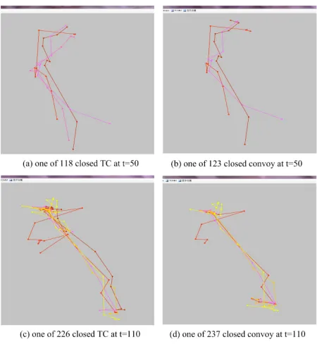
while CMC finds out 51 closed Convoys including 3 current closed convoys. When t=110, CTraStream discovers 50 closed trajectory clusters including 4 current closed trajectory clusters, while CMC finds out 61 closed convoys in-cluding 4 current closed convoys. As shown in Fig. 4, two closed convoys mined by CMC on data 1 lose a closely moving object compared with the correspond-ing trajectory clusters discovered by CTraStream. And Fig. 5(a) and Fig. 5(b) demonstrate the same situation on data 2. Fig. 6(a) and 7(a) show two current closed trajectory clusters on data 3 and data 4 respectively, and Fig. 6(b) and 6(b) show corresponding current closed convoys. The trajectory clusters dis-covered by CTraStream contain more relative time information compared with the convoys discovered by CMC. Fig. 6(c) and 6(d) depict respectively a closed trajectory cluster and two closed convoys on data 3. Obviously, CMC divides a group movement into two convoys. In conclusion, compared with CMC, the trajectory clusters discovered by CTraStream are closer to real movement track of moving objects with respect to the same parameters.
Fig. 4.Effectiveness comparison between CTraStream and CMC on data 1
6.3. Efficiency
Scalability. Next, a running time test is carried out on four datasets to verify
Fig. 5.Effectiveness comparison between CTraStream and CMC on data 2
Fig. 7.Effectiveness comparison between CTraStream and CMC on data 4
M inLns=3 on data1 and data 2,e=150,M inLns=3 on data 3,e=40,M inLns=4 on data 4. The running time of CTraStream in each time interval unit is reported in Fig. 8, in which the running time on data 1, data 3 and data 4 refer to left y-axis, and the running time on data 2 refers to right y-axis. The results show that the running time in every time interval unit fluctuates smoothly within a small range with increase or decrease in timestamp. And the results also demon-strate that our algorithm have a good scalability. In addition, Statistics on the experimental results shows that average clustering time of CTraStream for a line segment is about 0.42 ms, 0.64 ms, 0.42 ms and 0.3 ms on data 1, data 2, data 3 and data 4, respectively.
Efficiency comparison. With increase in received trajectory points, the
re-Fig. 8. Clustering time of CTraStream during each time interval unit on four datasets
Fig. 9.Comparisons of clustering time of CTraStream, CMC, and TCMM on four
datasets
Fig. 10.Efficiency of CTraStream, CMC and TCMM w.r.t.eon four datasets
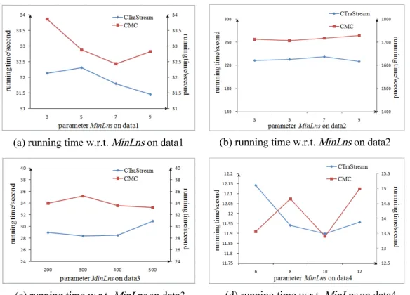
6.4. Parameter Sensitivity
Fig. 11.Efficiency of CTraStream and CMC w.r.t.M inLnson four datasets
7.
Conclusion
Discovering trajectory clusters from trajectory data stream is challenge, and ex-isting solutions to related problems are ineffective in processing data stream. This paper proposes a trajectory data stream clustering algorithm based on density, CTraStream, to extract all closed trajectory clusters from trajectory data streams online. CTraStream considers the incremental trajectories of mass moving objects as line segment streams. In the first stage, a density based line segment stream clustering algorithm is presented and a set of l-s-clusters is obtained at end of current time interval. In the second stage, a TC-tree is main-tained to store all closed trajectory clusters, an is updated according to the set of l-s-clusters by performing the update rules.
Acknowledgments.This work is supported by National Natural Science Foundation of China (No. 61172049, 61003251), National High Technology Research and Develop-ment Program of China (863 Program)(No. 2011AA040101), Doctoral Fund of Ministry of Education of China (No. 20100006110015), Project of Beijing Municipal Science and Technology Commission (Z111100054011078), the 2012 Ladder Plan Project of Beijing Key Laboratory of Knowledge Engineering for Materials Science (No. Z121101002812005), and construction project of Beijing Municipal Commission of Education.
References
1. Alexander Hinneburg, D.A.K.: An efficient approach to clustering in large multime-dia databases with noise. In: Proceedings of the 4th International Conference on Knowledge Discovery and Data Mining. pp. 58–65. AAAI Press, New York, USA (1998)
2. C. Piciarelli, G.F.: On-line trajectory clustering for anomalous events detection. Pat-tern Recognition Letters 27(15), 1835–1842 (2006)
3. Christian S. Jensen, Dan Lin, B.C.O.: Continuous clustering of moving objects. IEEE Transactions on Knowledge and Data Engineering 19(9), 1161–1174 (2007) 4. Gaffney, S., R.A.S.P.C.S., Ghil, M.: Probabilistic clustering of extratropical cyclones
using regression mixture models. Climate Dynamics 29(4), 423–440 (2007) 5. Gaffney, S., Smyth, P.: Trajectory clustering with mixtures of regression models. In:
Proceedings of the 5th International Conference on Knowledge Discovery and Data Mining. pp. 63–72. ACM Press, San Diego, California (1999)
6. Hwang, S.-Y., L.Y.H.C.J.K..L.E.P.: Mining mobile group patterns: A trajectory-based approach. In: Proceedings of 9th Pacific-Asia Conference on Knowledge Discovery and Data Mining. pp. 713–718. Springer-Verlag, Berlin, Heideberg (2005)
7. J., Yuan, Y.Z.C.Z.W.X.X.X.G.S.Y.H.: T-drive: driving directions based on taxi trajecto-ries. In: Proceedings of the 18th SIGSPATIAL International Conference on Advances in Geographic Information Systems. pp. 99–108. ACM Press, New York, USA (2010) 8. Jae-Gil Lee, J.H.: Trajectory clustering: A partition and group framework. In: Pro-ceedings of ACM SIGMOD 2007 International Conference on Management of Data. pp. 593–604. ACM press, Beijing, China (2007)
9. Jae-Gil Lee, Jiawei Han, X.L.H.G.: Traclass: Trajectory classiffication using hier-archical region-based and trajectory-based clustering. Proceedings of the PVLDB Endowment 1(1), 1081–1094 (2008)
10. Jeungy H, Yiu Man Lung, Z.X.J.C.S.e.a.: Discovery of convoys in trajectory databases. Proceedings of the VLDB Endowment 1(1), 1068–1080 (2008)
11. Joachim Gudmundsson, Marc van Kreveld, B.S.: Efficient detection of motion pat-terns in spatio-temporal data sets. In: Proceedings of the 13th International Sym-posium of ACM Geographic Information Systems. pp. 250–257. ACM Press, New York, USA (2004)
12. Jung-Im Won, Sang-Wook Kim, J.H.B.J.L.: Trajectory clustering in road network en-vironment. In: Proceedings of IEEE Symposium on Computational Intelligence and Data Mining, 2009. pp. 299–305. IEEE Press, Nashville, TN (2008)
14. Lu-An Tang, Yu Zheng, J.Y.J.H.: On discovery of traveling companions from stream-ing trajectories. In: Proceedstream-ings of IEEE 28th International Conference on Data En-gineering, 2012. pp. 186–197. IEEE Press, Washington, USA (2012)
15. M., N.: Clustering methods for spatio-temporal data. Univ. of Pisa, Italy (2002), phD thesis
16. M. Ankerst, M. Breunig, H.P.K., J, S.: Optics: Ordering points to identify the cluster-ing structure. In: Proceedcluster-ings of ACM SIGMOD 1999 International Conference on Management of Data. pp. 49–60. ACM press, Pennsylvania, USA (1999)
17. MacQueen, J.: Some methods for classi?cation and analysis of multivariate obser-vations. In: Proceedings of the Fifth Berkeley Symposium on Mathematical Statis-tics and Probability. pp. 281–297. University of California Press, Berkeley, California (1967)
18. Martin Ester, Hans-Peter Kriegel, J.S.e.a.: A density-based algorithm for discover-ing clusters in large spatial databases with noise. In: Proceeddiscover-ings of the 2nd In-ternational Conference on Discovery and Data Mining. pp. 226–231. AAAI press, Portland, OR (1996)
19. Nanni M., P.D.: Time-focused clustering of trajectories of moving objects. Journal of Intelligent Information Systems 27(3), 267–289 (2006)
20. Sigal Elnekave, Mark Last, O.M.: Incremental clustering of mobile objects. In: Pro-ceedings of IEEE 23rd International Conference on Data Engineering Workshop. pp. 585–592. IEEE Press, DC, USA (2007)
21. Slava Kisilevich, Florian Mansmann, M.N.S.R.: Spatio-temporal clustering: a survey. In: Oded Z. Maimon, L.R. (ed.) Data Mining and Knowledge Discovery Handbook, LLC, vol. 6, pp. 855–874. New York : Springer (2010)
22. T., B.: Network- based generator of moving object. Institute of Angewandte Pho-togrammetric and Geoinformatik (2005), [Online]. Available: http://iapg.jade-hs.de-/personen/brinkhoff/generator/
23. USDA: The starkey project. Oregon Department of Fish and Wildlife, US (1996), [Online]. Available: http://www.fs.fed.us/pnw/starkey/
24. Wei Liu, Yu Zheng, S.C.J.Y., Xie, X.: Discovering spatio-temporal causal interac-tions in traffic data streams. In: Proceedings of the 17th ACM SIGKDD international conference on Knowledge discovery and data mining, 2011. pp. 1010–1018. ACM Press, New York, USA (2011)
25. Y., Zheng, Y.C.X.X.W.Y.M.: Geolife2.0: A location-based social networking service. In: Proceedings of the 2009 Tenth International Conference on Mobile Data Man-agement: Systems, Services and Middleware. pp. 357–358. IEEE Press, Washing-ton, USA (2009)
26. Yifan Li, Jiawei Han, J.Y.: Clustering moving objects. In: Proceedings of the 10th International Conference on Knowledge Discovery and Data Mining. pp. 617–622. ACM Press, Seattle, Washington (2004)
27. Zhenhui Li, Jae-Gil Lee, X.L.e.a.: Incremental clustering for trajectories. In: Proceed-ings of 2010 International Conference on Database System For Advanced Applica-tions. pp. 32–46. Springer LNSS, Tsukuba, Japan (2010)
Yanwei Yu,PhD candidate at the School of Computer and Communication
Qin Wang,Professor at the School of Computer and Communication Engineer-ing, University of Science and Technology Beijing. Her research interest covers wireless sensor networks, wireless localization, data mining, and computer ar-chitecture.
Xiaodong Wang,Master student of University of Science and Technology
Bei-jing. His main research interest is trajectory data mining.
Huan Wang,Undergrad student of University of Science and Technology
Bei-jing. His main research interest is trajectory data mining.
Jie He,PhD, faculty at the School of Computer and Communication
Engineer-ing, University of Science and Technology Beijing. His research interest covers indoor positioning techniques and wireless sensor networks.

![Fig. 3. An example of TC-Tree during time interval [t1, t3].](https://thumb-us.123doks.com/thumbv2/123dok_us/1179018.1620552/12.612.148.469.370.527/fig-example-tc-tree-time-interval-t-t.webp)