AN EXTREMELY SIMPLE OPERATION
FOR DRASTIC PERFORMANCE
ENHANCEMENT OF GENETIC
ALGORITHMS FOR ENGINEERING
DESIGN OPTIMIZATION
M.H. Imam
Department of Civil Engineering Umm Al-Qura University, Makkah, Saudi Arabia
Imran A. Tasadduq
Department of Computer Engineering Umm Al-Qura University, Makkah, Saudi Arabia
Abstract
For significant performance enhancement of GA, we introduce a new and simple operation with the name Trans-addition involving binary addition of selected chromosome to Pseudo-blank chromosomes. A male Pseudo-blank has all but one of its bits set to zero. Its 2’s complement is the female. Trans-addition forces smallest possible change to each decision variable. The probability of such a change in canonical GA is quite low. Only the fittest chromosome performs Trans-addition with all Pseudo-blanks. It satisfies a natural behavior of higher opportunities of reproduction for the fittest. Trans-addition does not interfere with regular GA operations but only supplements. The implementation, named “Trans-GA”, is based on the representation of real-valued decision variables in terms of variable integer increments and user-specified accuracy. Our results clearly prove that Trans-GA outperforms the canonical GA in reliability and convergence rate by a wide margin. The presented GA implementation suits Engineering Design Optimization problems involving integer, real and mixed decision variables.
Keywords: Chromosome Trans-addition Genetic Algorithm Trans-GA Optimization Pseudo-blank
chromosome
1. Introduction
Vol. 2(11), 2010, 6630-6645
GA’s are not only an integral part of MA’s implementations but are still in wide use among engineers in all fields of engineering and multi-disciplinary optimization [Rajkumar et. al., (2008); Paulinas and Usinskas, (2007); Paszkowics, (2009); El-Mihoub et. al. (2006)]. Google Scholar reports 2300 papers concerning GA applications published in 2009. Many engineers and researchers use MATLAB toolbox and there are several software packages that have been developed with built-in GA. GA’s have been commonly used in solving both CO and DO problems. However, a wide class of the real-world Engineering Design Optimization (EDO) problems belongs to a particular type of DO. Such EDO problems in fact have continuous design space but they don’t need solutions with the accuracy of a large number of decimal places as is common in CO problems. Such solutions are not practical and issues of availability and manufacturability arise. The dimensions of most mechanical or electrical components or structural elements can only be specified with an accuracy that is practical. The actual values of the decision variables may be real but they belong to a finite discrete set. An example is the set of values of the diameters of rods used in a truss structure. The diameters may be chosen from a user-specified finite set of values, e.g., {1.00, 1.25, 1.50, 1.75...}. The values are real but discrete. In such cases of DO, a decision variable may be considered as an integer that acts as a pointer to the discrete values in the user-specified set. Most of the EDO problems based on analytical principles are of this type. Such EDO problems do not require a floating point representation and can be binary coded in terms of the number of increments. The user-specified value of the increment determines the type of accuracy or precision required. The published MA, PSO or other EA’s do not suit such problems and become too complex to implement real world EDO problems. To address this issue, a simple GA implementation is needed that satisfies the requirements of such EDO problems and at the same time improves the performance significantly.
This paper presents a binary-coded GA implementation for achieving drastic performance enhancement to a canonical or conventional GA (CGA) at no additional computational cost. This objective is achieved by introducing a new GA operation in CGA. The introduction of this new operation is meant to solve three problems in binary-coded GA implementations. First, it provides a mechanism to impose smallest possible variation in each decision variable in each generation. In contrast, a binary-coded CGA or any of its variants has very low probability of bringing small changes to a decision variable even when the crossover and mutation probabilities are set to high. Gaussian mutation instead of uniform mutation has been in common use in various GA software packages to overcome this problem in real-coded GA’s. However, no solution to this problem for binary-coded GA’s has been proposed in the literature. Secondly, the presented implementation is meant to remedy the problem of Hamming cliff [Gen and Chang, (2000)] that occurs in binary coded GA’s. Thirdly, it provides a unified approach for all types of EDO problems regardless whether the decision variables are real or integer or mixed.
The new GA operation introduced in this paper has been named “Trans-addition”. Trans-addition operates on a set of chromosomes called “Pseudo-blank” chromosomes. The GA implementation incorporating this operation will be referred to as Trans-GA. The implementation involves chromosome encoding by representing each real-valued decision variable in terms of integer number of increments and user-specified accuracy parameter. This implementation is also meant to patch all existing GA implementations seamlessly without affecting any of the existing operations of GA or any of its variants including MA.
The paper is organized in eleven sections including this introduction. Section 2 gives a brief overview of CGA. Before introducing the new operation to the reader, the issue of managing the accuracy of decision variables is discussed in Section 3. This issue is common to CGA and Trans-GA. Section 4 presents the idea of Pseudo-blank chromosomes. In Section 5, Trans-addition operation is described. Mathematical description of Trans-addition for a general class of problems is presented in Section 6. This is followed by a description of test problems in Section 7. Performance comparison measures used for evaluating the presented implementation are discussed in Section 8 and simulation results are presented in Section 9. Reasons for effectiveness of the proposed algorithm are discussed in Section 10. Section 11 gives the conclusions and directions of further research.
2. Canonical GA
Canonical Genetic Algorithm
1 initialize population 2 evaluate population
3 while termination criterion not reached 4 select solutions for next population 5 perform crossover and mutation
6 evaluate population
Fig. 1 Canonical Genetic algorithm structure [Srinivas and Patnaik, (1994)]
3. Decision variable Accuracy
Almost all algorithms, especially GA, rely on the accuracy of the digital computer involved. For the Trans-GA implementation presented in this paper, all operations take place on binary bits which in fact is in accordance with the original GA implementation concept. However, when representing a set of decision variables with a bit string (the chromosome), the question of how to maintain the required accuracy of a decision variable arises. Infinite accuracy is not possible and too high an accuracy is not practical. In EDO problems, the user must specify the required accuracy for each decision variable based upon the requirement of a particular problem being solved. Therefore, within the framework of GA, user-specified accuracy for each decision variable must be implemented. This is done through a simple step described in the following.
Let
i be an ith individual such that
i
S
where S is the solution space andS
, and
is a set of real numbers. Let the upper bound on the solution space for ith individual beU
i and the lower bound beL
i. Since the proposed algorithm is primarily for solving EDO problems, these upper and lower bounds are user-specified. Further, let the desired accuracy for the ith individual be represented by
i. Since an individual would always lie in the rangeU
i
L
i, it is easy to show that the value of an individual at any stage during the algorithm can be represented as:i i i
i
L
N
[1]
Here
N
irepresents the number of increments required in order to represent the individual at a particular stage in the algorithm. This approach not only gives the freedom of specifying the desired accuracy but it also simplifies the encoding of chromosomes as only the increments, i.e., onlyN
ineed to be encoded. The number of bits required to encodeN
i can be computed using the following relationship:1
1
log
INT
2
i i i i
L
U
N
[2]
The “INT” operator in the above equation picks up the integer part of the number and discards the fractional part. Now the bit string value represents the number of increments that need to be added to
L
iin order to determine the value of an individual in the given solution space. The implementation presented in this paper is based on the above equations to represent the accuracy of the decision variables.4 Pseudo-Blank Chromosomes
Vol. 2(11), 2010, 6630-6645
Table 1 Example of Pseudo-blank chromosomes
Male Pseudo-blank 000000!00000001 000001!00000000
Female Pseudo-blank 000000!11111111 111111!00000000
4. Trans-Addition
In genetics, “Trans-addition” is a term used for a special type of combination operation that takes place between two entities such as water molecule with some other molecule [Ozhan and Alpertunga, (2007)]. The proposed new GA operation has some resemblance to “Trans-addition” and therefore we named it Trans-addition. The purpose of this operation is to force the minimum possible variation in the value of each decision variable. This variation is equal to the user-specified increment for each decision variable. This is achieved by a binary addition operation between a part of a selected chromosome representing one of the decision variables and the corresponding part of “Pseudo-blank” chromosome. Trans-addition of a chromosome with a male Pseudo-blank causes a particular decision variable to increase its value by the user-specified increment and thus brings the minimum possible variation forcefully in each generation. Similarly Trans-addition of a chromosome with a female Pseudo-blank causes a decrease in the value of a particular decision variable equal to the user-specified increment. This operation therefore, increases the probability of the smallest change in the values of each decision variable to 100%; a phenomenon that CGA and all its published variants as well as Memetic algorithms lack. This operation forces a chromosome to keep converging towards the highest possible fitness it can attain whenever mutation and crossover are unable to do it.
Concerning the selection for Trans-addition, it is argued that the opportunity of Trans-addition (like reproduction or nourishment in a natural uncontrolled environment) will be enjoyed only by the fittest. Based on this principle, only the fittest chromosome of the population is given the opportunity to perform Trans-addition with all Pseudo-blanks. This makes the algorithm simple and at the same time the natural phenomenon of privileged opportunities for the fittest is maintained.
Since, the fittest chromosome of a generation performs Trans-addition with N male chromosomes and N female chromosomes, 2N offspring are born where N is the number of decision variables. Thus, the trans-addition pool has 2N+1 chromosome other than the 2N Pseudo-blanks. The fittest of these 2N+1 chromosomes in the Trans-addition pool is returned to the population and others are discarded. This process is not a local search but just a mechanism to bring the smallest possible variation in the values of all decision variables therefore the implementation may not be classified as a Memetic algorithm. Actually a Memetic can be based on this new GA with Trans-addition and may become much more effective.
The algorithm starts with the calculation of the chromosome bit string size based on the user-specified accuracy and range (lower and upper bounds) for each decision variable using Eq. (2) of Section 3. Then, the pool of Pseudo-blanks is populated with N male and N female Pseudo-blank chromosomes of the calculated size. Each Pseudo-blank is different from the other. This step in the implementation of Trans-GA, of populating the pool of Pseudo-blanks, is not in a loop. Once the pool of Pseudo-blanks is populated, it is preserved in the original state through all generations so the fittest chromosome comes and performs Trans-addition with all Pseudo-blanks that are the same in all generations.
The next step of the algorithm is random generation of initial population using user specified accuracy and range for each decision variable. As explained in Section 3, the binary bit string corresponding to each decision variable has the lowest decimal value equal to zero and the highest value equal to the number of maximum increments required so that Eq. (1) gives the upper bound imposed on the decision variable. The randomly generated chromosomes represent the set of decision variables such that the resulting decimal value of each decision variable is within the specified range when calculated using Eq. (1). The randomly generated chromosomes are of the same length as the Pseudo-blank chromosomes.
Next, the operation of Trans-addition takes place between the fittest chromosome of the population and each of the Pseudo-blank pairs. Thus, there are two Trans-addition operations. Once, the fittest chromosome and a male Pseudo-blank are the parents. A child is born. Next, the fittest chromosome and the female counterpart Pseudo-blank are the parents. Another child is born. This operation is continued until Trans-addition has been performed with all Pseudo-blank pairs.
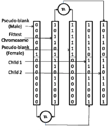
The Trans-addition operation for an optimization problem involving two variables is shown in Fig. 2. In this Figure, the operation has been shown separately for male and female Pseudo-blanks. This operation is not the canonical binary addition between two chromosome bit strings. It is binary addition of one part of a bit string to the corresponding part of another bit string and hence the name Trans-addition. In Fig. 2, variable 1 is shown encoded using 6 bits while variable 2 is encoded using 8 bits indicating that the range between the lower and upper bounds of the two different decision variables is different. In this figure, the fittest chromosome selected from the population goes through Trans-addition operation with a pair of Pseudo-blanks and produces two children.
Fig. 2 Trans-addition for a two variable problem
The fittest of the newly born offspring due to Trans-addition if better than the fittest of the previous generation returns from the Trans-addition pool to the population for the next generation operations. It may be noted that the fittest chromosome from the Trans-addition pool does not replace the weakest but the fittest of the previous generation. If the fittest of Trans-addition replaces the weakest of the population, the population will soon be dominated by the similar chromosomes and the capability of finding the global optimum will be decreased. After the Trans-addition loop, the next step is to perform conventional crossover and mutation operations of CGA. The complete algorithm is shown in Fig. 3.
Trans-GA Algorithm
1 initialize population 2 evaluate population
3 generate male and female Pseudo-blank chromosomes 4 while termination criterion not reached
5 select solutions for next population
6 perform Trans-addition between fittest chromosome and each of the Pseudo-blank chromosomes and generate two children
7 perform crossover and mutation
8 evaluate population
Fig. 3 Structure of Trans-GA
5. Mathematical Formulation of the Problem
A typical optimization problem can be mathematically formulated as follows:
Maximize (or Minimize)
F
(
X
)
Subject to:
, , 1 ;
, , 1 ;
0 ) (
j U L
n i X
j j j i
where
Vol. 2(11), 2010, 6630-6645
iables design var of
number Total
s constraint inequality
of number Total
iable design var th
of Value
iable design var th
on bound Upper
iable design var th
on bound Lower
s Constraint )
(
function Objective )
(
iables design var of
Vector
n
j j U
j L
X X F X
j j j i
The possible solutions to such problems are represented in the search space as bit strings of 0’s and 1’s – called chromosomes, obtained by converting the decision variables into binary numbers. As was mentioned in the previous section, a chromosome has an associated fitness value indicating how good the solution satisfies the optimization problem at hand. Of course, the higher the fitness value the better is the solution.
In a typical genetic algorithm, constraints can be handled in a number of ways – some have been discussed in [Holland, (1975)]. One of the ways could be to only keep the feasible solution and discard others. However, this may lead to the following problems:
1) Generating an initial population that only has feasible solution is a difficult task
2) It would get extremely difficult to find the global minima if many infeasible solutions are rejected
We therefore take the following approach. The infeasible solutions are kept in the space but we apply constraint violation penalties as follows:
100
,
max
)
(
X
F
F
F
i i P
[4]
where
contraints
Violated
applied
been
has
penalty
after the
alue
Function v
PF
Here the violated constraints includ the violation of the upper and lower bounds on the decision variables because such violations may take place in binary coded GA.
6. Test Problems
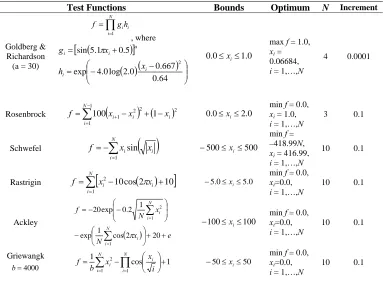
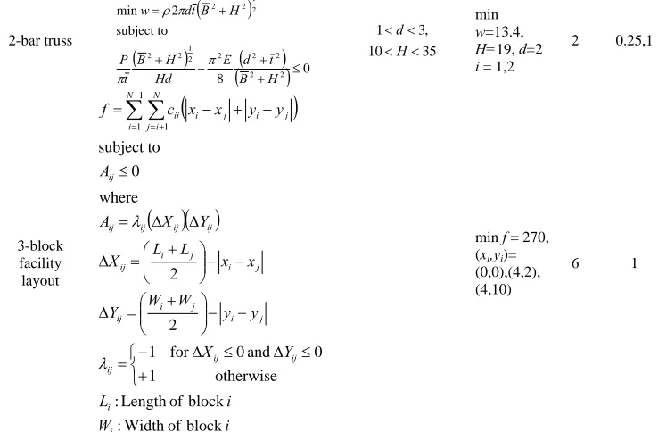
Performance of Trans-GA is evaluated by comparing it with CGA on eight test problems. The first six are well known test problems [Koumousis and Katsaras, (2006)] that have been used to evaluate and compare various GA implementations. The two other problems are EDO problems. First one is a well known structural optimization problem of 2-bar truss [Fox, (1971)] and the second problem is a combinatorial optimization problem of facility layout optimization [Planopt, 2010]. Although the Trans-GA has been proposed for EDO problems that don’t require an accuracy of large number of decimal places, it will be tested with the six well known benchmark problems of continuous domain optimization just to make sure of its robustness. An additional constraint on the comparison will be imposed by comparing the binary coded Trans-GA with real-coded CGA. This puts Trans-GA in a more severe test because binary real-coded CGA are known to have weaknesses like Hamming Cliff that do not occur in real-coded GA. Table 3 gives details of these test problems.
7. Performance Comparisons
Four types of comparison measures will be used to compare the performance. All these comparison measures are based on the closeness of the fitness value to the known optimum value. The closeness is normalized so that the comparisons are plotted on the same scale. The normalized closeness and the four comparison measures are described below:
a. Normalized Closeness
e
c
where,
F
*F
ˆ
;
F
*e
and is an arbitrary small number that has been usedto avoid division by zero in case F* is zero or close to zero. We have used a value of = 0.01 that works well for all functions given in Table 3.b. Performance Comparison Measures
The four performance comparison measures used to compare Trans-GA with CGA are as follows:
(1) Measure 1: The best and mean of the normalized closeness obtained from 100 optimization runs are compared.
(2) Measure 2: Number of function evaluations to obtain a given closeness is compared.
(3) Measure 3: Quality of solution in terms of the closeness is compared. This is done through plots that show the closeness obtained versus the optimizations runs. This graph will be called “Performance Comparison Graph” or PCG because it provides the best measure to evaluate and compare the performance of an algorithm.
(4) Measure 4: Trans-GA and CGA with Gaussian mutation are compared. This comparison is provided to show that the binary-coded Trans-GA gives a better performance than the real-coded CGA with Gaussian mutation which is known to give superior results.
8. Results
Results of 100 optimization runs with different random starting seeds are presented. Each optimization run has the same starting seed for both Trans-GA and CGA. All other parameters are kept the same for both the algorithms as shown in Table 4. Statistical comparisons based on the four measures are described in the following.
Table 3 Details of test functions used for simulations
Test Functions Bounds Optimum N Increment
Goldberg & Richardson (a = 30)
N i i ih g f 1 , where
64 . 0 667 . 0 0 . 2 log 0 . 4 exp 5 . 0 1 . 5 sin 2 i i a i i x h x g 0 . 1 0 .0 xi
max f = 1.0,
xi = 0.06684,
i = 1,…,N
4 0.0001
Rosenbrock
1 1 2 2 2 1 1 100 N i i i
i x x
x
f 0.0xi2.0
min f = 0.0,
xi = 1.0,
i = 1,…,N
3 0.1
Schwefel
N i i i x x f 1
sin 500xi500
min f = –418.99N,
xi = 416.99,
i = 1,…,N
10 0.1
Rastrigin
N i i i x x f 1 2 10 2 cos
10 5.0xi5.0 min xi=0.0, f = 0.0,
i = 1,…,N
10 0.1
Ackley
x e
N x N f N i i N i i
20 2 cos 1 exp 1 2 . 0 exp 20 1 1 2 100 100 ximin f = 0.0,
xi=0.0,
i = 1,…,N
10 0.1
Griewangk
4000
b cos 1
1 1 1 2
N i i N i i i x x bf 50xi50 min xi=0.0, f = 0.0,
i = 1,…,N
Vol. 2(11), 2010, 6630-6645
2-bar truss
08 subject to 2 min 2 2 2 2 2 2 1 2 2 2 1 2 2 H B t d E Hd H B t P H B t d w 35 10 , 3 1 H
d min w=13.4,
H=19, d=2
i = 1,2
2 0.25,1 3-block facility layout
i W i L Y X y y W W Y x x L L X Y X A A y y x x c f i i ij ij ij j i j i ij j i j i ij ij ij ij ij ij N i N ij ij i j i j
block of Width : block of Length : otherwise 1 0 and 0 for 1 2 2 where 0 subject to 1 1 1
min f = 270, (xi,yi)= (0,0),(4,2), (4,10)
6 1
Table 4 GA parameters used for simulations
GA Parameter Value
Selection Stochastic uniform
Mutation Uniform (pm = 0.01) Crossover Single-point (pc = 0.8) Elitism 2
a. Comparison Measure 1 (Best and Mean)
As mentioned earlier, the performance comparison measure 1 compares the best, and the mean of the normalized closeness obtained from 100 optimization runs. This comparison is shown in Table 5. It is obvious from Table 5 that in all cases, the best of the 100 optimization runs of Trans-GA gets to the 100% normalized closeness (i.e. the known optimum fitness) whereas CGA obtains 100% closeness in one case only. In two cases i.e., Rastrigin and Ackley, the performance of CGA is extremely poor. Similarly, for all the test problems, the mean obtained by Trans-GA is much better than that obtained by CGA. A question may arise about how many times an algorithm gets to the best. This has been answered in Table 6 which shows clear superiority of Trans-GA.
b. Comparison Measure 2 (Function Evaluations)
Table 5 Best and mean closeness
Test Functions
Normalized closeness (%)
Best Mean CGA Trans-GA CGA Trans-GA
1) Goldberg & Richardson 98.97 100.00 88.18 94.72
2) Rosenbrock 86.10 100.00 15.47 54.93
3) Schwefel 99.58 100.00 97.92 99.95
4) Rastrigin 17.42 100.00 2.26 66.32
5) Ackley 29.42 100.00 10.27 100.00
6) Griewangk 98.65 100.00 92.62 100.00
7) Truss Design 100.00 100.00 95.77 98.36
8) FLP 83.09 100.00 53.55 85.58
Table 6 Frequency of occurrence of best closeness
Test Functions
Frequency of occurrence
90% closeness 100% closeness
CGA Trans-GA CGA Trans-GA
1) Goldberg & Richardson 40 78 0 42
2) Rosenbrock 0 53 0 53
3) Schwefel 0 100 0 99
4) Rastrigin 0 66 0 66
5) Ackley 0 100 0 100
6) Griewangk 75 100 0 100
7) Truss Design 95 96 23 81
8) FLP 0 59 0 32
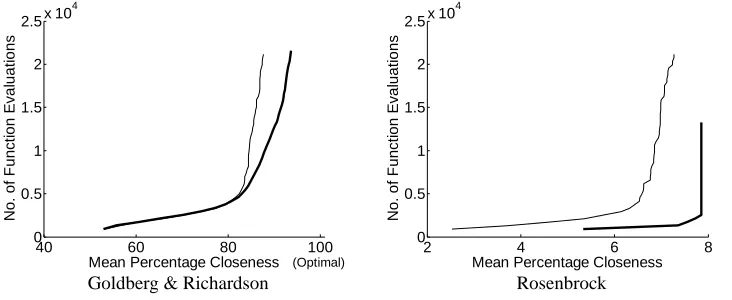
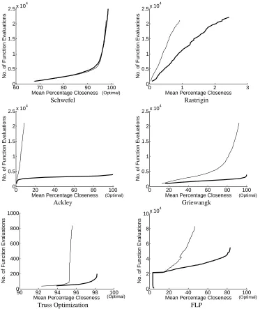
It is obvious from the plots shown in Fig. 4 that Trans-GA does not introduce any extra computational cost because its computational efficiency is higher. In the case of Goldberg & Richardson function, CGA and Trans-GA both require almost the same number of function evaluations for obtaining 80% closeness. However, for obtaining a closeness of more than 80%, Trans-GA’s superiority is very obvious from the graph. Schwefel is the only function in which CGA and Trans-GA have about the same number of function evaluations but CGA does not get to 100% closeness whereas Trans-GA obtains 100% closeness. In all other cases, it is obvious from the graphs that Trans-GA requires significantly fewer function evaluations than CGA.
40 60 80 100
0 0.5 1 1.5 2 2.5x 10
4
Mean Percentage Closeness
N
o
. of F
u
n
c
ti
on E
v
al
uati
ons
(Optimal)
2 4 6 8
0 0.5 1 1.5 2 2.5x 10
4
Mean Percentage Closeness
N
o
. of F
u
n
c
ti
on E
v
al
uati
ons
Vol. 2(11), 2010, 6630-6645
60 70 80 90 100
0 0.5 1 1.5 2 2.5x 10
4
Mean Percentage Closeness
N
o
. of F
u
n
c
ti
on E
v
al
uati
ons
(Optimal)
0 1 2 3
0 0.5 1 1.5 2 2.5x 10
4
Mean Percentage Closeness
N
o
. of F
u
n
c
ti
on E
v
al
uati
ons
Schwefel Rastrigin
0 20 40 60 80 100
0 0.5 1 1.5 2 2.5x 10
4
Mean Percentage Closeness
N
o
. of F
u
n
c
ti
on E
v
al
uati
ons
(Optimal)
0 20 40 60 80 100
0 0.5 1 1.5 2 2.5x 10
4
Mean Percentage Closeness
N
o
. of F
u
n
c
ti
on E
v
al
uati
ons
(Optimal)
Ackley Griewangk
90 92 94 96 98 100
0 200 400 600 800 1000
Mean Percentage Closeness
N
o
. of F
u
nc
ti
on E
v
al
uati
ons
(Optimal) 0 20 40 60 80 100
0 2 4 6 8 10x 10
4
Mean Percentage Closeness
N
o
. of F
u
n
c
ti
on E
v
al
uati
ons
(Optimal)
Truss Optimization FLP
Fig. 4 Function evaluations as a function of normalized closeness
c. Comparison Measure 3 (PCG)
0 20 40 60 80 100 70
75 80 85 90 95 100
No. of Runs
P
e
rc
enta
ge C
los
enes
s
*
*Optimal 0 20 40 60 80 100
70 75 80 85 90 95 100
No. of Runs
P
e
rc
enta
ge C
los
enes
s
*
*Optimal
(a) Unsorted PCG (b) Sorted PCG
Fig. 5 An example of sorted and unsorted PCG
It is obvious that the sorted PCG is much more meaningful in comparing two algorithms and therefore we will present the comparisons using the sorted PCG’s.
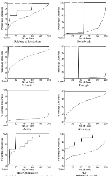
The sorted PCG’s of all the test problems are shown in Fig. 6. Each plot shows the result of 100 independent runs. As mentioned earlier, closeness of 100% indicates that the known optimum has been reached.
Superiority of Trans-GA is clearly visible from Fig. 6. For Goldberg & Richardson, Trans-GA is superior for each optimization run in one to one correspondence with the sorted closeness. It may be noted that this does not mean that starting from a given seed, Trans-GA will always be better in closeness. In Rosenbrock function, for about 50 sorted runs, the performance is about the same but for the other half, the performance of Trans-GA is clearly and significantly superior. Also, Trans-GA obtains the known optimum in about 50 of the hundred runs whereas CGA never gets to the known optimum. For Schwefel function, Trans-GA for almost all the optimization runs obtains the known optimum and is drastically superior to CGA. For Rastrigin function, CGA and Trans-GA perform poorly in about 35% of runs but for the rest 65% of the runs Trans-GA gets to the 100% closeness whereas CGA is way behind. Ackley function is an example where CGA is extremely poor and Trans-GA has improved it drastically by obtaining 100% closeness for 100 runs. Grienwanck function almost behaves the same way as Schwefel function except that Trans-GA obtains 100% closeness for all the 100 runs. The Truss Optimization problem and the FLP problem both show the same trend with clear superiority for Trans-GA.
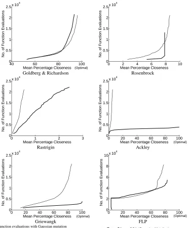
d. Comparison Measure 4 (Comparison with Gaussian Mutation)
Since Gaussian mutation is known to improve the performance of GA’s, it is worth comparing it with Trans-GA. In comparing Trans-GA and a CGA with Gaussian mutation, it may be noted that Gaussian mutation is only applicable to real-coded GA. It does not work with binary-coded GA. Real-coded GA already has advantages over binary-coded GA’s. Since Trans-GA is a binary coded GA, comparing it with real-coded GA employing Gaussian mutation is putting Trans-GA to the most severe test. The results of such a comparison are shown in Fig. 7 and Fig. 8. In these figures, the results of Schwefel function and the Truss Optimization problem are not included because they cannot be solved using Gaussian mutation due to the constraints imposed.
Vol. 2(11), 2010, 6630-6645
0 20 40 60 80 100
70 75 80 85 90 95 100
No. of Runs
P
e
rc
enta
ge C
lo
s
enes
s
*
*Optimal 0 20 40 60 80 100
0 20 40 60 80 100
No. of Runs
P
e
rc
enta
ge C
lo
s
enes
s
*
*Optimal
Goldberg & Richardson Rosenbrock
0 20 40 60 80 100
94 95 96 97 98 99 100
No. of Runs
P
e
rc
enta
ge C
lo
s
enes
s
*
*Optimal 0 20 40 60 80 100
0 20 40 60 80 100
No. of Runs
P
e
rc
enta
ge C
lo
s
enes
s
*
*Optimal
Schwefel Rastrigin
0 20 40 60 80 100
0 20 40 60 80 100
No. of Runs
P
e
rc
enta
ge C
lo
s
enes
s
*
*Optimal 0 20 40 60 80 100
80 85 90 95 100
No. of Runs
P
e
rc
enta
ge C
lo
s
enes
s
*
Ackley Griewangk
0 20 40 60 80 100
85 90 95 100
No. of Runs
P
e
rc
enta
ge C
lo
s
enes
s
*
*Optimal 0 20 40 60 80 100
20 40 60 80 100
No. of Runs
P
e
rc
enta
ge C
lo
s
enes
s
*
*Optimal
Truss Optimization FLP
40 60 80 100 0
0.5 1 1.5 2 2.5x 10
4
Mean Percentage Closeness
N
o
. of F
u
n
c
ti
on E
v
al
uati
ons
(Optimal)
0 2 4 6 8 10
0 0.5 1 1.5 2 2.5x 10
4
Mean Percentage Closeness
N
o
. of F
u
n
c
ti
on E
v
al
uati
ons
Goldberg & Richardson Rosenbrock
0 1 2 3
0 0.5 1 1.5 2 2.5x 10
4
Mean Percentage Closeness
N
o
. of F
u
n
c
ti
on E
v
al
uati
ons
0 20 40 60 80 100
0 0.5 1 1.5 2 2.5x 10
4
Mean Percentage Closeness
N
o
. of F
u
n
c
ti
on E
v
al
uati
ons
(Optimal)
Rastrigin Ackley
0 20 40 60 80 100
0 0.5 1 1.5 2 2.5x 10
4
Mean Percentage Closeness
N
o
. of F
u
n
c
ti
on E
v
al
uati
ons
(Optimal)
0 20 40 60 80 100
0 2 4 6 8 10x 10
4
Mean Percentage Closeness
N
o
. of F
u
n
c
ti
on E
v
al
uati
ons
(Optimal)
Griewangk FLP
Fig. 7: Function evaluations with Gaussian mutation
9. Why Trans-addition is more effective?
The poor performance of CGA is not something new. Due to its poor performance other algorithms like Memetic algorithms and PSO have been developed. Now from comparisons presented in the previous sections and from the very obvious results of Trans-GA’s significantly better performance, we confirm the reason of the poor performance of CGA. The only difference between the CGA and Trans-GA implementations compared is the new GA operation of Trans-addition. Therefore, the reason of the poor performance of CGA is merely its inability (or very low probability) to make smallest possible change in the decision variables. Trans-GA becomes so good merely because the new GA operation introduced in this paper overcomes this problem and forces the smallest possible variations in the values of the decision variables in each generation.
Vol. 2(11), 2010, 6630-6645
0 20 40 60 80 100
70 75 80 85 90 95 100
No. of Runs
P
e
rc
enta
ge C
lo
s
enes
s
*
*Optimal 0 20 40 60 80 100
0 20 40 60 80 100
No. of Runs
P
e
rc
enta
ge C
lo
s
enes
s
*
*Optimal
Goldberg & Richardson Rosenbrock
0 20 40 60 80 100
0 20 40 60 80 100
No. of Runs
P
e
rc
enta
ge C
lo
s
enes
s
*
*Optimal 0 20 40 60 80 100
0 20 40 60 80 100
No. of Runs
P
e
rc
enta
ge C
lo
s
enes
s
*
*Optimal
Rastrigin Ackley
0 20 40 60 80 100
60 70 80 90 100
No. of Runs
P
e
rc
enta
ge C
lo
s
enes
s
*
*Optimal 0 20 40 60 80 100
40 50 60 70 80 90 100
No. of Runs
P
e
rc
enta
ge C
lo
s
enes
s
*
Griewangk FLP
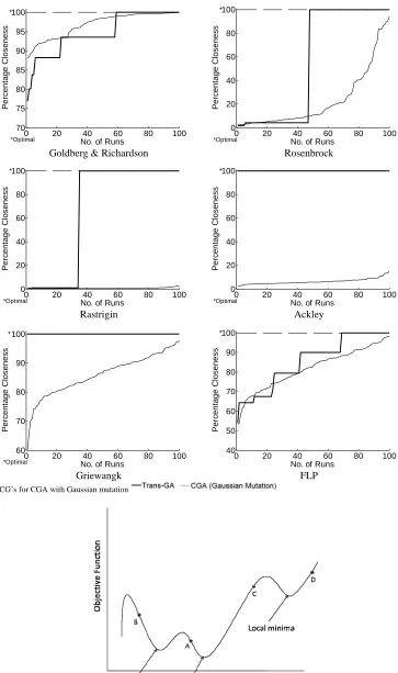
Fig. 8: PCG’s for CGA with Gaussian mutation
While minimizing the function using CGA, let us assume that the algorithm reaches point A on the curve. Since the probability of small change in the value of a decision variable is low in CGA, it may take a large number of crossovers to be able to reach the optimum point. Now compare the solution to the problem through Trans-GA where an additional operation of Trans-addition is incorporated. Since Trans-addition brings minimum possible variations in the values of the variables, after reaching point A, the algorithm will gradually and steadily move the point towards the global minimum and achieve it. This is another explanation of why the introduction of Trans-addition enhances the performance of the algorithm.
10.Conclusions
A new GA operation called Trans-addition has been introduced for achieving significant performance enhancement to binary coded GA’s. It is an extremely simple GA operation and can be patched seamlessly to the canonical GA or any of its variants. The presented GA implementation based on Trans-addition has been given the name of “Trans-GA”. The implementation specially addresses the requirement of Engineering Design Optimization problems by representing the decision variables in terms of user-specified accuracy. This makes the presented Trans-GA implementation capable of solving all types of Engineering Design Optimization problems involving real, integer or mixed type of decision variables. The proposed implementation can be used as the base algorithm for MA’s. It does not involve any additional computation cost but instead reduces the number of computations.
The proposed implementation brings significant and even drastic enhancements because it addresses the root cause of poor performance of binary-coded CGA i.e. the low probability of small variations in the decision variable. At the same time, by imposing the smallest variation in each decision variable in each generation, it overcomes the Hamming Cliff problem.
Superiority of Trans-GA is established by using four different performance comparison measures on a set of test problems consisting of six well-known test problems and two simple EDO problems. Trans-GA outperforms canonical GA by a wide margin in all the measures for all the test problems. In the first performance measure, the best and mean of the normalized closeness to the known optima and the frequency of occurrence of the best are compared. The best of Trans-GA runs always gets to 100% closeness (i.e. obtains the known optima) for all test problems while canonical GA achieves the known optimum in only one case and in some cases the best closeness is extremely poor, for example, 17% for Rastrigin function and 29% for Ackley function. The mean obtained by Trans-GA is also indicative of its superior performance. In five of the test problems the mean of Trans-GA runs is close to the known optimum (greater than 90% closeness with 100% in two of the eight problems). The frequency of occurrence of the known optima is also an important criterion. Trans-GA obtains frequency of occurrence of the known optima ranging from 100 out of 100 in two test problems to a minimum of 32 out of 100. In contrast the frequency of occurrence to the known optima for CGA is mostly zero out of 100.
The second performance measure compares the number of function evaluations required to achieve a given mean closeness to the known optimum. In all cases Trans-GA requires fewer function evaluations except for Schwefel function that has identical number of function evaluations. In some cases like Ackley function and Truss Optimization problem, Trans GA has drastically fewer function evaluations than CGA. The third performance measure is based on an idea of a “Performance Comparison Graph” or a PCG. PCG is a sorted plot of the closeness obtained in each run. In all cases, Trans-GA exhibits clearly superior performance.
The fourth performance measure puts Trans-GA to the most severe test. It is a comparison of binary coded Trans-GA to real-coded CGA with Gaussian mutation. Again, in almost all the test problems, the performance of Trans-GA in terms of number of function evaluations or through the PCG’s can be clearly seen to be significantly or drastically superior.
Trans-GA with such an overwhelming performance can be used for all types of EDO problems and has the potential to replace all variants of CGA that are being used in MATLAB and other EDO applications. Its potential for being a base algorithm for MA’s seems very promising and is therefore a very good direction of future research. Further research may also be undertaken to explore the characteristics of Trans-GA by applying it to more real-world problems from various disciplines.
References
[1] Beyer, H. G., and Schwefel, H. P.: Evolution strategies. Natural Computing. 1, 3–52 (2002) [2] Davis, L.: Handbook of genetic algorithms. New York: Van Nostrand Reinhold (1991)
[3] El-Mihoub, Tarek A., Adrian A. Hopgood, Lars Nolle, Alan Battersby: Hybrid Genetic Algorithms: A Review. Engineering Letters, 13(2), (2006)
[4] Fox, Richard L.: Optimization Methods for Engineering Design. Massachusetts: Addison-Wesley, (1971) [5] Gen, M. and Runwei Chang: Genetic Algorithms and Engineering Optimization. John Wiley, New York (2000)
[6] Goldberg, D. E., and Voessner, S.: Optimizing global-local search hybrids. In W. Banzhaf et al. (Eds.), Proceedings of the Genetic and Evolutionary Computation Conference’99 (pp. 220–228). San Mateo, CA: Morgan Kaufmann (1999)
Vol. 2(11), 2010, 6630-6645
[8] Herrera, F., Lozano, M., and Verdegay, J. L.: Tackling real-coded genetic algorithms: Operators and tools for the behavioral analysis. Artificial Intelligence Review. 12(4), 265–319 (1998)
[9] Holland, J.H.: Adaptation in Natural and Artificial Systems. Univ. of Michigan Press, Ann Arbor, Mich. (1975)
[10] Kennedy, J., and Eberhart, R. C.: Particle swarm optimization. In Proceedings of the IEEE International Conference of Neural Networks. pp. 1942–1948 (1995)
[11] Koumousis, Vlasis K., Christos P. Katsaras: A saw-tooth genetic algorithm combining the effects of variable population size and reinitialization to enhance performance. IEEE Trans. Evol. Comput. 10(1), 19–28, Feb. (2006)
[12] Krasnogor, N., and Smith, J. E.: A tutorial for competent memetic algorithms: Model, taxonomy, and design issue. IEEE Transactions on Evolutionary Computation. 9(5):474–488 (2005)
[13] Lee, C.-Y., and Yao, X.: Evolutionary programming using mutations based on the Levy probability distribution. IEEE Transactions on Evolutionary Computation. 8(1):1–13, (2004)
[14] Lozano, M., Herrera, F., Krasnogor, N., and Molina, D.: Real-coded memetic algorithms with crossover hill-climbing. Evolutionary Computation, 12(3):273–302 (2004)
[15] Merz, P.: Memetic algorithms for combinatorial optimization problems: Fitness landscapes and effective search strategies. Ph.D. Thesis, University of Siegen, Germany (2000)
[16] Molina, D., Herrera, F., and Lozano, M.: Adaptive local search parameters for real-coded memetic algorithms. In Proceedings of the 2005 IEEE Congress on Evolutionary Computation. pp. 888–895 (2005)
[17] Molina, D., Manuel Lozano, Carlos Garc´ıa-Mart´ınez , Francisco Herrera: Memetic Algorithms for Continuous Optimisation Based on Local Search Chains. Evolutionary Computation. 18(1), 27–63, Januray, (2010)
[18] Moscato, P. A.: Memetic algorithms: A short introduction. In D. Corne, M. Dorigo, and F. Glower (Eds.), New ideas in optimization (pp. 219–234). New York: McGraw-Hill (1999)
[19] Moscato, P. A.: On evolution, search, optimization, genetic algorithms and martial arts: Towards Memetic algorithms. Technical Report. Caltech Concurrent Computation Program Report 826, Caltech, Pasadena, CA (1989)
[20] Ong, Y. S., Lim, M.-H., Zhu, N., and Wong, K. W.: Classification of adaptive memetic algorithms: A comparative study. IEEE Transactions on Systems, Man, and Cybernetics, 36(1):141–152 (2006)
[21] Özhan, Gül, Buket Alpertunga: Polymorphism of microsomal epoxide hydrolase. International Journal of Molecular Biology, Biochemistry and Gene Technology, Jan. (2007)
[22] Paszkowicz, Wojciech: Genetic Algorithms, a Nature-Inspired Tool: Survey of Applications in Materials Science and Related Fields. Materials and Manufacturing Processes, 24(2), 174–197 (2009)
[23] Paulinas, Mantas and Andrius Ušinskas: A Survey of Genetic Algorithms Applications for Image Enhancement and Segmentation. Information Technology and Control. 36(3), (2007)
[24] Rajkumar, N., Timo Vekara, and Jarmo T. Alander: A Review of Genetic Algorithms in Power Engineering. In Tapani Raiko, Pentti Haikonen, and Jaakko Väyrynen, editors, AI and Machine Consciousness, Proceedings of the 13th Finnish Artificial Intelligence Conference STeP 2008, pages 15–32, Espoo (Finland), 20.-22. August 2008. FAIS, Helsinki.
[25] Renders, J. M., and Flasse, S. P.: Hybrid methods using genetic algorithms for global optimization. IEEE Transactions on Systems, Man, and Cybernetics, 26(2):243–258 (1996)
[26] Srinivas, M. and Lalit M. Patnaik.: Genetic Algorithms: A Survey. IEEE Computer, 27(6), 17–26, (1994)
[27] Storn, R., and Price, K. V.: Differential Evolution—A simple and efficient heuristic for global optimization over continuous spaces. Journal of Global Optimization. 11(4), 341–359, (1997)