S O F T W A R E
Open Access
Kinematic analysis of diastolic function
using the freely available software Echo
E-waves
–
feasibility and reproducibility
Martin G. Sundqvist
1, Katrin Salman
2, Per Tornvall
1and Martin Ugander
2*Abstract
Background:Early diastolic left ventricular (LV) filling can be accurately described using the same methods used in classical mechanics to describe the motion of a loaded spring as it recoils, a validated method also referred to as the Parameterized Diastolic Filling (PDF) formalism. With this method, each E-wave recorded by pulsed wave (PW) Doppler can be mathematically described in terms of three constants: LV stiffness (k), viscoelasticity (c), and load (x0). Also, additional parameters of physiological and diagnostic interest can be derived. An efficient software application for PDF analysis has not been available. We aim to describe the structure, feasibility, time efficiency and intra-and interobserver variability for use of such a solution, implemented in Echo E-waves, a freely available software application (www.echoewaves.org).
Results:An application was developed, with the ability to open DICOM files from different vendors, as well as rapid semi-automatic analysis and export of results. E-waves from 20 patients were analyzed by two investigators. Analysis time for a median of 34 (interquartile range (IQR) 29–42) E-waves per patient (representing 63 %, IQR 56–79 % of the recorded E-waves per patient) was 4.3 min (IQR 4.0–4.6 min). Intra-and intraobserver variability was good or excellent for 12 out of 14 parameters (coefficient of variation 2.5–18.7 %, intraclass correlation coefficient 0.80–0.99).
Conclusion:Kinematic analysis of diastolic function using the PDF method for Doppler echocardiography implemented in freely available semiautomatic software is highly feasible, time efficient, and has good to excellent intra-and interobserver variability.
Keywords: Diastolic function, Echocardiography, Kinematic analysis, Software
Background
Diastole, the time during which the ventricles of the heart fill with blood, is conventionally assessed by measuring various blood flow velocities, time intervals, ratios of velocities, and dimensions of chambers and walls of the heart [1]. The investigator then tries to fit these measure-ments with a theoretical and empirical body of knowledge constituting part of our understanding of left ventricular (LV) mechanics and hemodynamics. As such, the conven-tional method of assessing diastolic function lacks a unifying theory. Improving our ability to investigate diastolic function is of importance not only as it is vital to our understanding of cardiac function in health and
disease, but also in order to better approach diagnostics and treatment options in the increasingly recognized con-dition of heart failure with preserved ejection fraction. We aim to describe an alternative strategy for assessing diastole, and a software implementation for this method that is ready for use in clinical research.
During the cardiac cycle, the LV contracts during systole, whereby the volume of blood in the LV decreases. During early diastole, the LV recoils, leading to an increase in the volume of blood in the LV, with blood entering the LV through the mitral valve. In the absence of aortic regurgitation or shunts, the velocity of blood flow through the mitral valve during early diastole will be the same as the velocity of volume expansion of the LV, and hence the velocity of LV recoil. The velocity of transmitral blood flow can readily be measured by pulsed wave (PW) Doppler echocardiography. It has * Correspondence:[email protected]
2Department of Clinical Physiology, Karolinska Institutet, and Karolinska University Hospital, SE-171 76 Stockholm, Sweden
Full list of author information is available at the end of the article
been shown that the velocities of early diastolic transmi-tral blood flow, and thus LV recoil, can be accurately de-scribed as a case of damped harmonic motion [2]. Damped harmonic motion is a part of the analytical framework describing motion in classical mechanics, and can been used, among other things, to describe the recoil of a spring. From this framework one can derive a mathematical expression that describes velocity as a function of time in terms of three constants, namely stiffness (k), viscoelasticity, or energy loss, (c), and load (x0). By curve fitting the velocity profile of the PW
Doppler signal of the E-wave to the mathematical ex-pression, the constants can be obtained. The theoretical framework describing LV filling in this manner has been termed the parameterized diastolic filling (PDF) formalism [2]. Using gold standard high fidelity invasive hemodynamic measurements, the stiffness constantk has been shown to have a close linear rela-tionship with LV diastolic stiffness [3]. In the same manner, it has been shown that the influence of the damping constant c can be used to formulate an accurate estimate of the invasively determined time constant of isovolumic pressure decay, tau [4].
Furthermore, a load independent index of diastolic filling, called M, can be calculated by examining the relationship between the peak driving force and the peak resistive force of filling at different levels of load [5]. Furthermore, clinical studies have illustrated the utility of the PDF method in characterizing clinical disease including diabetes [6, 7], hypertension [8], as well as prognosis in congestive heart failure [9]. A brief overview of the PDF parameters is given in Table 1, and further details are given in the Appendix. In summary, this unified approach to studying early diastolic filling narrows the gap between clinical echocardiography and classical mechanics, and also promises new insights into different pathological states as well as basic cardiac physiology. However, a user-friendly solution enabling PDF analysis of echo-cardiographic DICOM images and output of results in a fashion optimized for clinical research use has not been available [10]. Therefore, we aim to describe the structure, feasibility, time efficiency and intra-and interobserver variability for use of such a solution, implemented in Echo E-waves, a freely available soft-ware application.
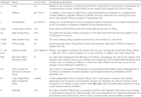
Table 1Overview of PDF parameters
Parameter Name Unit (SI unit) Physiological description
x0 Load cm Related to the load that is compressing the elastic myocardium at end systole, a prerequisite for a restoring force to arise. Closely related to the velocity time integral (VTI) of the E-wave.
k Stiffness g/s2(N/m) LV rigidity, or the extent to which the LV resists deformation in response to an applied force. Linearly related to chamber stiffness [3] (dP/dV), and thus influences the restoring force that drives early diastolic filling. Increased in hypertension [8].
c Viscoelasticity g/s (N∙s/m) Energy loss or damping of LV recoil, caused by impaired relaxation and increased viscoelasticity of the myocardium. Increased in diabetes [6] and hypertension [8].
Vmax E-wave peak velocity m/s Peak velocity of blood flow across the mitral valve during early LV filling.
kx0 Peak driving force mN The peak force driving LV filling, analogous to the peak atrioventricular pressure gradient [14]. The product ofkandx0,
cVmax Peak resistive force mN The force resisting filling at peak transmitral flow. The product ofcand Vmax.
1/2kxo 2
Filling energy mJ Stored potential elastic energy from systole that generates rapid early LV filling. Increased in hypertension [8].
c2−4k orβ
Damping index g2/s2(kg∙N/m) Reflects the balance between the factors driving and resisting left ventricular filling. Values <−900 g2/s2are a strong predictor of 1-year mortality in elderly with heart failure [9]. KFEI Kinematic filling
efficiency index
% An index that characterizes the efficiency of LV filling. Calculated as the ratio of the velocity time integral of the actual E-wave to the velocity time integral of a PDF model-predicted ideal E-wave contour with no resistance to filling (c= 0) but the same stiffness (k) and load (x0) as for the original E-wave. Reduced in diabetes [7].
tau Time constant of isovolumic pressure decay
ms Tau is used to characterize LV filling based on time-resolved high fidelity invasive measurements of LV pressure. Increased in impaired relaxation. Can be approximated by combination of PDF parameters [4].
M Load independent
index of diastolic filling
unitless A load independent index of diastolic filling, which is decreased in patients with diastolic dysfunction and increased LV end-diastolic pressure [5]. Describes the ratio of change in peak driving force to change in peak resistive force (Δkx0/ΔcVmax), calculated after acquiring E-waves under varying loading conditions.
B Intercept mN An index of diastolic filling that is increased in patients with diastolic dysfunction and increased LV end-diastolic pressure [5]. Mathematically, the y-axis intercept of the relationship between the peak driving and resistive forces from E-waves acquired under varying loading conditions.
Implementation
The program, Echo E-waves, is freely available for download at www.echoewaves.org [11]. It is imple-mented in the MATLAB® release 2015a (Mathworks, Natick, Massachusetts, USA) environment for Win-dows (64-or 32-bit architecture). In the following sec-tion we describe the structure and funcsec-tionality of the program. For analysis of inter-and intraobserver vari-ability, sets of E-waves with visually moderate to good quality were selected from 20 patients undergoing echocardiography as part of ongoing clinical studies on adults with acute myocardial infarction with or without obstructive coronary artery disease, and excluding patients with significant valvular disease. The studies were approved by the Regional Ethical Review Board in Stockholm, Sweden, and all subjects provided written informed consent. All echocardio-graphic acquisitions were performed on Vivid E9 scanners (GE, Horten, Norway). The Echo E-waves program was run on an Intel® Core i5™ 2500 K pro-cessor with a NVIDIA® GeForce® GTX 670 graphics card and the 64-bit version of Windows 7.
Echocardiographic image acquisition
The program can analyze PW Doppler echocardio-graphic images of transmitral flow acquired in the same manner as is recommended by clinical guide-lines [12]. However, some adjustments are suggested to ensure improved accuracy in analysis. A horizontal sweep speed of 100 mm/s is recommended, as lower sweep speeds lead to a substantial loss of temporal resolution. A sweep speed of 150 mm/s or 200 mm/s is also acceptable. However, in our experience these sweep speeds make the visual recognition of the shape of the E-wave somewhat more difficult, since they are less commonly used clinically. The program currently reads DICOM images from GE, Philips, Siemens and Acuson systems. When using a GE or Philips system, the user can export a cine recording of Doppler data stretching over several screen widths as a single DICOM multi frame file. A method for this is described in on the program website (www. echoewaves.org). From all the systems above, single frame DICOM image files can also be loaded. For the purposes of testing the intra-and interobserver vari-ability, 20 echocardiographic exams collected during ongoing clinical trials were selected. The exams were performed by four dedicated sonographers, all with at least 8 years of experience with clinical echocardiog-raphy. A 3.5 mm sample volume was placed at the tips of the mitral leaflets, and PW Doppler recordings were performed both during free breathing and after cessation of the Valsalva maneuver.
Loading and visualization of Doppler data from DICOM images
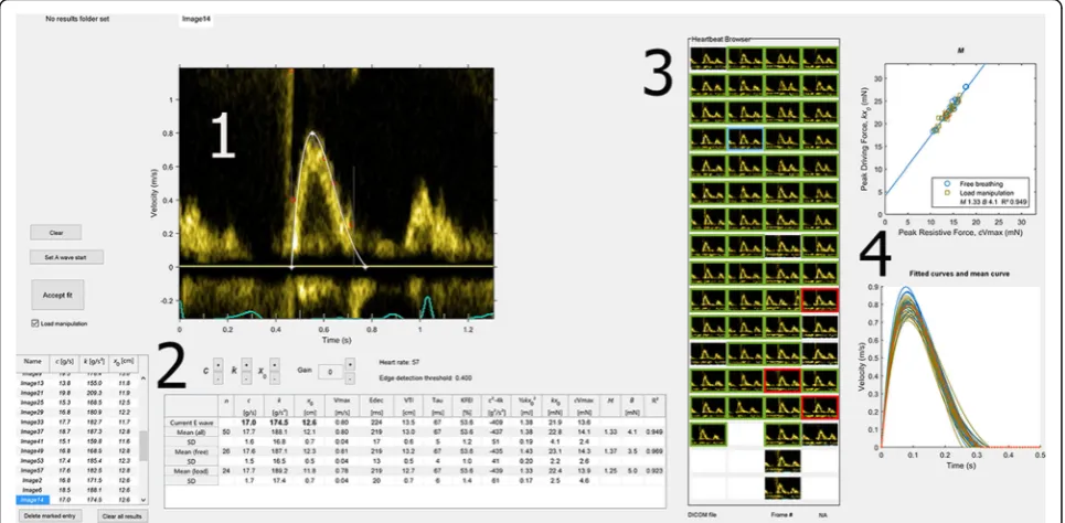
Using DICOM metadata, the Doppler region of the image is automatically identified and displayed with correct time and velocity scaling. For ease of overview, the contents of the folder are displayed as thumbnails in the Heartbeat Browser, also enabling navigation of the data set using mouse or keyboard input. Extended (cine) recordings of Doppler registrations from GE and Philips scanners are automatically cropped to one image per cardiac cycle. In order to facilitate the detection of the part of the Doppler signal constituting the E-wave, the user can change color maps, gain settings and apply contrast stretching. Currently, the program does not load the contents of folders with a mix of single frame and cine DICOM files. The graphical user interface is described in Fig. 1.
Detection of the velocity profile
In the data structure of a DICOM image, Doppler data is represented as a two dimensional matrix of numbers, with each matrix index corresponding to a velocity at a given point in time. In these images, the horizontal axis of the image is time in seconds, and the vertical axis is velocity in meters per second. The value at a given matrix index indicates the brightness of the pixel at the corresponding position in the image, and the brightness corresponds to the amount of blood travelling at that given velocity at that point in time. For the purpose of detecting the velocity profile, the program searches each column (i.e. each time point) of the image from the top down for the first pixel having a brightness higher than or equal to a user defined threshold level, matching each time point with a velocity. However, as the Doppler re-cording is susceptible to noise, and due to the presence of non E-wave signal, the algorithm has been optimized by taking into account pre-existing knowledge of how the velocity profile of the E-wave can be differentiated from Doppler signal not originating from the E-wave. For instance, velocity at the moment when flow is about to begin must be zero. Furthermore, we can assume that there must be an upper limit to the velocity difference between two time points a few milliseconds apart. The algorithm accordingly discards a detected velocity that differs too much from the previous velocity. Discarded velocities are displayed for reference and transparency as to the behavior of the algorithm.
can lead to substantial differences in the constants resulting from curve fitting. In many cases, the exact position of the onset of flow can be difficult to ascertain visually at first glance. However, the velocity profile during the acceleration time is often quite distinct, and if close attention is paid to how different starting points affect the visual correspondence of the PDF curve to the underlying Doppler data of the acceleration time and the upper, often well defined part of the E-wave, a convin-cing position for the starting point can be identified in effectively all cases. Positioning of the end point must take into account the various non-E-wave Doppler signals that frequently occur during the deceleration phase. A good curve fit will often be achieved if the end point is set at approximately 75 % of the total E-wave duration and typically at less than 50 % of the maximum wave velocity. In the case of partial overlap of the E-and the A-wave, the user must examine the E-wave to see if it is of sufficient duration to determine where it would have ended had there been no overlap between the E-and the A-wave. Typically, this is not possible when the crossover point between the E-and the A-wave occurs at a velocity is above 50 % of the maximum velocity of the E-wave. The program contains no par-ticular feature to guide the user in this process, but using the alternative method to curve fitting described below can often make the task easier. We recommend excluding E-waves from analysis when there is an overlap with the A-wave at greater than 50 % of the
nature of the Doppler acquisition (noise and non-E-wave signal during the deceleration time and diastasis), they are based on empirically determined parameters. In our experience, using them will lead to a faster and more intuitive curve fitting workflow, in that the sensitivity to the problems mentioned above will be reduced. These fitting settings should be viewed as improvements to speed of effectively obtaining a visually acceptable fit, and not as changes to the PDF model per se. If the user so chooses, they can be disabled individually.
Curve fitting and adjustment of the fitting algorithm input
The paired time-velocity data obtained during detection is used as input to a native curve fitting function of MATLAB, which employs the Levenberg-Marquardt algorithm, a standard algorithm for solving non-linear least square problems. After curve fitting, the constants
c, k, and x0are obtained with values that, when used as
input to an expression of velocity as a function of time, would yield the closest match to the originally detected velocity profile. This calculated curve is displayed as an overlay to the original Doppler image, along with the result of the velocity profile detection algorithm for visual confirmation. After display of the fitted curve, the user can adjust the start and end points of the velocity profile detection time interval, as well as the threshold for detection, resulting in an automatic update of the fitted curve. These adjustments can be made by clicking and dragging with the mouse, or by using keyboard shortcuts. No measures of goodness of fit for the E-wave are displayed. Mathematically, the curve fitting process will produce an excellent fit in nearly all cases, and dif-ferences in e.g. sum of squared errors cannot be used to decide if an adjustment to a fit will result in a physiolo-gically more accurate fit. Rather, we have found that vis-ual assessment is the most reliable and useful method for assessing the appropriateness of a given fit.
Automatic detection and curve fitting
In order to facilitate curve fitting of data sets comprised of large numbers of E-waves, a semi-automatic algo-rithm for curve fitting several E-waves has been imple-mented. The user must first set the starting point and adjust the settings so that the first E-wave is fit in an acceptable manner. The program stores the part of the image corresponding to the start of this user-defined E-wave as a template. The template is then used to find the starting point of the E-wave on the subsequent images using normalized cross correlation. The velocity profile detection algorithm described above is then run from this starting time point to either 1/3 of a cardiac cycle, or to the time point where velocity has fallen below 35 % of the peak velocity of the E-wave. The
detected velocities are used for curve fitting as described above. The resulting parameters are compared to the mean of the previously obtained parameters, and if any parameter of the current E-wave deviates more than 40 % from the mean of the previous, the program dis-cards the fit and moves on to the next E-wave. Usage of this automated method can speed up analysis, however, it requires close scrutiny of the obtained results.
Quality control
In order to review produced results, and also facilitate the identification of anomalies, the results are displayed simul-taneously in multiple fashions. The numerical values of the constantsc, k, and x0are displayed in a list, and the
mean of the constants and the derived parameters are also displayed. Furthermore, the calculated curve for each E-wave is displayed in a graph, where each curve is select-able. Each E-wave is also displayed as a selectable marker in a plot of peak driving force vs. peak resistive force. Selecting an E-wave in any of these displays retrieves and displays the corresponding E-wave with its fitted curve, which can then be adjusted or deleted if the user so chooses.
Alternative method to curve fitting
It has been shown that the curves yielded by applying the mathematics of damped harmonic motion to Doppler E-wave velocity profiles can be fully described in terms of unique combinations of their acceleration and deceleration times and peak velocities [13]. In other words, each unique combination of the constantsc,k, andx0also has a unique
combination of acceleration and deceleration time and peak velocity. As a consequence of this, the constants for an E-wave can be calculated if these two time intervals and the velocity are known. As an alternative to fitting the full data set of velocities, it is thus possible to use just these three measurements. In the program, this is implemented both as a primary way of producing a curve, and as a method for adjusting a previously obtained curve. The user can pro-duce a curve by marking the start, peak velocity and end points. For any curve, regardless of if it was produced by curve fitting or this alternative method, the start, peak and end points are manually adjustable by dragging them with the mouse, enabling an easy user interface for adjusting the shape of the curve, which is updated in real time.
Export of data
Saving of images and graphs is also possible. It is also possible to copy the results to the computer’s memory clipboard and paste them into a program of choice. The program also stores the part of the DICOM images containing the Doppler data as well as any results of curve fitting and user interaction, so that images and/ or curve fits for a given set of DICOM files can be retrieved, reviewed and/or edited at a later time. Saving in this manner also enables full optional anonymiza-tion, leaving the saved file without any trace of patient or source file identification. These data files are created in the native .mat format of MATLAB. When saving the results of an analyzed case, it also possible to desig-nate a results folder, which will save all results to a common space, and also append each case to a file (.xlsx or.txt) with the means and standard deviations of all constants for each case, effectively creating a study database.
Statistical analysis
All statistical analyses were performed in MATLAB release 2015a (Mathworks, Natick, Massachusetts, USA). The basic PDF constants and the derived parameters were analyzed as mean values for each patient. The coefficient of variation (CV) for the difference between measure-ments, intraclass correlation coefficient, and percentage difference with standard deviation were calculated and presented as needed. The CV was calculated as the
standard deviation of the mean differences between analyses divided by the mean and expressed as a percent. Durations of analysis and numbers of analyzed E-waves are reported as median and interquartile range (IQR).
Results
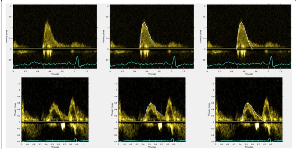
Representative results of the performance of the velocity profile detection algorithm and the corresponding fitted curves are shown in Fig. 2.
For each patient, 34 (29–42) E-waves were analyzed. Thus, 63 (56–79) % of the recorded E-waves per patient were deemed to be of sufficient quality to perform curve fitting with visually acceptable results. The time for analyzing one patient case was 4.3 (4.0– 4.6) minutes. These timings were calculated by letting the automatic fitting algorithm analyze all E-waves, after which the investigator reviewed the whole set, making adjustments as necessary. The median, range and interquartile range of the analyzed parameters are shown in Table 2. For the peak driving force, the per patient mean range was 8 mN.
Inter-and intraobserver repeatability
The results for observer variability are presented in Table 3. Overall, inter-and intraobserver reliability was good to excellent. The investigators were free to discard E-waves for which a visually convincing fit was not pos-sible to obtain. Limiting analysis to only those E-waves
Fig. 2Representative examples of Doppler velocity profile edge detection and the resulting fittedcurvesfor two different patients (top
andbottom, respectively).Leftpanels: original Doppler images.Midpanels: detected edges of the velocity profiles inwhite.Rightpanels: fittedcurves(white). PDF parameters for thetop row:c17.3 g/s,k135 g/s2x
for which both investigators had accepted fits yielded similar results. The notable exception to this was the parameters M and B. For M, interobserver variability was high when all fitted E-waves were considered. Dis-carding those E-waves for which one of the investigators had not provided a result yielded a substantial improve-ment. By comparison, the interobserver variability for B was substantial using both approaches.
Discussion
We have described how the freely available software ap-plication Echo E-waves can be used to analyze transmi-tral Doppler recordings in the PDF framework. The application can be used to obtain results in a timely fashion, and makes it feasible to investigate further usage of this approach to measuring and assessing diastolic function. Furthermore, intra -and interobserver reliability was good, with the exception of the load independent index of filling, M, and the interceptB. There may be several reasons for these findings. As it is defined, Mis the slope of a regression line describing the relationship between driving and resistive forces under different load-ing conditions. As for all linear regression slope values, the accuracy ofM can be disproportionately influenced by outliers, and the decision to include a particular E-wave can have a sizable impact onM. In order to allevi-ate the disproportionallevi-ate impact of potential outliers, one would prefer a data set with a wide variation in load, with a roughly equal spread of E-waves with regards to differences in loading conditions. In our population, using the load variation after the Valsalva maneuver, the per patient mean range of peak driving force was only 8 mN. By comparison, in the study by Shmuylovichet al,
the range was 30–40 mN, with load variation induced by varying the body position of the subjects using a tilt board and body positions ranging from head up 90° to head down 90° [5]. It seems likely that this larger load variation could lead to a more accurate assessment of
M, however, the present study is the first to analyze the inter-and intraobserver reliability regardless of loading conditions. It should also be noted that the optimal cut off values and ranges for usingMfor clinical or scientific work have yet to be determined. Other methods for in-ducing variations in load are worthy of exploration. Fur-thermore, the optimal number of E-waves necessary for reliable analysis is also worthy of further investigation. It should also be noted that we did not examine the test-retest variability. Future studies incorporating multiple examinations per subject are motivated in order to ad-dress the effects of user dependency in echocardio-graphic image acquisition on quantification of PDF measures.
To our knowledge, there is only one other publicly available software application for PDF analysis [10]. The advantages of Echo E-waves are the ability to analyze DICOM files directly without pre-processing or file conversion, general ease of use, ability to review, com-pare, quality control, and revise E-wave delineations in the program environment, semi-automatic fitting and efficient export of results in various formats. Further-more, Echo E-waves does not require installation of other software requiring licensing costs.
Conclusions
The software program Echo E-waves is freely available and can be used to quantify and investigate diastolic function and dysfunction using insights from classical mechanics in the PDF framework, producing results rapidly and reliably enough for application of this method for use in the cardiac imaging community.
Appendix
Mathematical details of the PDF framework
The equation describing the balance of forces in a damped harmonic oscillator is
md2x dt2þc
dx
dtþkx¼0: ð1Þ
In the PDF framework, inertia (m) is set to 1 g, with the other constants formulated on a per unit mass basis. The units of the other constants are g/s2 (N/m) for k and g/s (Ns/m) for c. In the analysis of E-waves, x will always be a negative number with the unit m, however as it basically describes a displacement or distance, and considering that typical values at the onset of motion (x0) are in the region of−0.1 m, we have chosen to
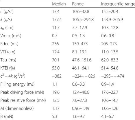
Table 2Results of PDF analysis in 20 patients
Median Range Interquartile range
c(g/s2) 17.4 10.6–32.8 15.5–20.4
k(g/s) 177.4 106.5–294.8 153.9–206.9
x0(cm) 11.7 7.7–17.9 10.3–12.8
Vmax (m/s) 0.7 0.5–1.3 0.6–0.8
Edec (ms) 236 139–473 205–273
VTI (cm) 12.4 8.1–19.1 11.0–13.5
Tau (ms) 70.1 47.6–151.6 62.0–83.3
KFEI (%) 53.0 46.1–64.1 51.4–54.8
c2−4k(g2/s2) −382 −224–−826 −295–−474
Filling energy (mJ) 1.1 0.6–3.3 0.9–1.4
Peak driving force (mN) 19.6 12.4–40.6 17.6–22.7
Peak resistive force (mN) 12.5 7.6–27.3 10.6–14.7
M (dimensionless) 1.17 0.96–1.49 1.06–1.26
B (mN) 5.3 1.6–9.7 4.1–6.7
present the results of x0 as a positive number with the
unit cm, for ease of reading. From the foundational equation (1), expressions describing the velocity of motion as function of time can be derived. For under-damped cases, defined byc2−4k< 0, the expression for velocity (v) as a function of time (t) is
v tð Þ ¼−kx0
ω exp
−c 2 t
sinð Þ;ωt ð2Þ
where
ω ¼
ffiffiffiffiffiffiffiffiffiffiffiffi 4k−c2 p
2 : ð3Þ
For overdamped cases, defined by c2−4k> 0, the expression is
v tð Þ ¼−kx0
β exp
−c 2 t
sinhð Þ;βt ð4Þ
where
Table 3Inter-and intraobserver variability
3A Intraobserver Interobserver
CV (%) Difference (%) SD ICC CV (%) Difference (%) SD ICC
c 13.2 12.6 9.8 0.80 11.6 9.8 6.1 0.92
k 9.3 9.1 7.3 0.93 14.0 9.0 8.3 0.88
x0 6.6 4.7 4.8 0.95 5.9 4.7 4.6 0.96
Vmax 5.1 3.3 4.0 0.98 4.0 3.0 2.6 0.99
Edec 11.1 7.6 7.5 0.92 11.8 9.1 6.2 0.93
VTI 6.0 4.1 4.2 0.96 5.3 4.3 3.4 0.97
Tau 11.7 8.9 8.4 0.88 13.3 10.2 6.7 0.91
KFEI 2.7 2.6 2.0 0.89 2.5 2.2 1.9 0.91
c2−4k 18.7 18.9 30.1 0.92 14.3 16.2 14.7 0.95
Energy 14.6 13.7 9.6 0.94 10.6 9.8 6.4 0.98
Peak driving force 10.7 9.8 8.1 0.92 10.6 8.1 6.0 0.95
Peak resistive force 14.6 13.5 10.6 0.85 12.9 10.6 7.2 0.93
M 15.3 12.1 8.3 0.51 23.7 17.7 20.8 0.16
B 44.7 39.5 32.6 0.37 51.1 37.0 38.7 0.32
3B Intraobserver Interobserver
CV (%) Difference (%) SD ICC CV (%) Difference (%) SD ICC
c 13.6 12.5 10.6 0.80 11.6 10.4 5.3 0.93
k 9.0 8.6 6.8 0.94 13.7 9.2 7.7 0.88
x0 5.5 3.9 4.8 0.96 5.5 4.3 4.5 0.96
Vmax 2.4 2.3 1.9 0.99 3.8 3.0 2.5 0.99
Edec 9.7 6.9 7.1 0.94 11.5 7.9 6.6 0.94
VTI 4.0 2.9 3.1 0.98 5.1 4.2 3.2 0.97
Tau 10.7 8.6 8.0 0.90 13.1 8.8 7.1 0.92
KFEI 2.9 2.6 2.3 0.88 2.6 2.4 1.8 0.91
c2−4k 17.9 15.8 25.0 0.93 12.7 13.1 11.9 0.96
Energy 16.0 14.2 11.0 0.93 10.9 9.7 6.5 0.98
Peak driving force 11.0 10.5 8.5 0.91 10.8 8.2 5.9 0.94
Peak resistive force 15.7 14.5 11.8 0.83 13.3 10.9 6.9 0.93
M 15.4 12.1 8.3 0.61 13.5 10.2 11.2 0.71
B 44.7 39.5 32.6 0.51 27.9 19.6 19.9 0.83
3A are the results obtained when observers were free to choose which E-waves to analyse from each set. 3B are the results obtained when comparing only those E-waves which both observers had analyzed. Forc2
β¼
ffiffiffiffiffiffiffiffiffiffiffiffi c2−4k p
2 : ð5Þ
For critically damped cases, defined byc2−4k= 0, the expression is
v tð Þ ¼−kx0t exp −c
2 t
: ð6Þ
Curve fitting the appropriate function to the time-velocity data obtained from the detection of the time-velocity profile results in a c, k, and x0 value for each E-wave.
Using these constants, the peak velocity (Vmax) can be calculated as the velocity at the time point of no acceler-ation or deceleracceler-ation. The energy available for filling at the onset of the E-wave is ½kx02[mJ]. For underdamped
cases, exact values for the deceleration time and area under the curve (velocity time integral, VTI) can be calculated, deceleration time being
DT¼π
ω−
1
ω tan−1
2ω
c ; ð7Þ
and VTI being the integral under the curve from the starting point t= 0 to the time point where the velocity reaches zero.
For overdamped and critically damped cases, velocity approaches zero asymptotically and thus an exact time point where the curve returns to zero velocity does not exist. However, an approximation can be formulated resembling the manner in which the deceleration time is measured in clinical echocardiography. Shmuylovich for-mulated this solution for the overdamped case [13]:
DT¼ 1ffiffiffi k
p γ
2y2eγ−y; ð8Þ
with
y¼ c
2pffiffiffik ; ð9Þ
and
γ¼ln 1þ
ffiffiffiffiffiffiffiffiffiffiffiffi 1−y−2
p
1−pffiffiffiffiffiffiffiffiffiffiffiffi1−y−2
!− 1 2pffiffiffiffiffiffiffi1−y−2
: ð10Þ
The fact that each E-wave can be described in terms of three constants, withc corresponding to impediment to recoil in a general sense, also makes it possible to calcu-late an E-wave free from the energy loss which a non-zero c entails. Setting c to zero, but using the k and x0
values from an actual E-wave, it is possible to compare the VTI and deceleration time of an ideal E-wave free from energy loss, with those of the actual E-wave. The ratio of the actual VTI to the ideal VTI is termed the kinematic filling efficiency index (KFEI) [7]. The
difference in E-wave duration between the actual and ideal E-wave is termed the relaxation component of the deceleration time (DTr), describing the prolongation of early filling due to imperfect relaxation and viscosity. DTr has been shown to have a close linear relationship withtaumeasured invasively [4].
From equation (1) the conditions at peak flow velocity (Vmax, whered2x
dt2¼0 andt=tpeak) can be stated as
cVmaxþkxtpeak ¼0; ð11Þ
implying that these forces are equal and of opposite direction. Assuming that the relationship between the force driving recoil at the onset of flow (kx0) and at peak recoil velocity (kxtpeak) is linear (having the form y = M’x + B’), equation (11) can be restated as
cVmaxþM0kx0þB
0
¼0; ð12Þ
from which follows that
kx0¼McVmaxþB: ð13Þ
Since equation (1) is applicable at all levels of load, equation (13) should be load independent as well, with
M describing the relationship between the driving and resistive forces of filling at different levels of load;M can thus be termed a load independent index of filling, and its load independency has been shown in human experi-ments [5].
Abbreviations
DICOM:Digital imaging and communications in medicine; KFEI: Kinematic filling efficiency index; LV: Left ventricle; PDF: Parameterized diastolic filling; PW: Pulsed Wave (Doppler)
Acknowledgements
The authors thank and acknowledge the following individuals for discussions, bug reports and/or other input into the development of the software: Sándor J Kovács PhD MD, Peter A Cain MBBS PhD, Ythan H Goldberg MD, Brett D Atwater MD, Emelie Mörtsell MD, and medical students Fahim Khan, David Megyessi, Mischa Flam, and Madeleine Turesson.
Funding
The studies from which the patients were selected were supported by grants from the Swedish Research Council, the Swedish Heart and Lung Foundation, Stockholm County Council ALF grant and Karolinska Institutet/ Stockholm County Council Strategic Cardiovascular Programme. The trials were performed without any relationships to industry.
Availability of data and materials
Project name: Echo E-waves
Project home page: www.echoewaves.org Operating system: Windows 32-/64-bit Programming language: MATLAB, Java Other requirements: MATLAB Runtime version 8.5
Restrictions: All publications containing data produced using Echo E-waves must clearly state this in the description of the study methods, and also reference the present software article.
Authors’contributions
MS participated in study design, designed and programmed the software, performed PDF analysis, statistical analyses and drafted the manuscript. KS performed PDF analysis for interobserver variability testing and participated in testing of the software. PT was responsible for the clinical studies from which patients were included into the study, and participated in study design and drafting of the manuscript. MU designed the study, participated in design and testing of the software, and drafted the manuscript. All authors have read and approved of the final manuscript.
Competing interests
The authors declare that they have no competing interests.
Consent for publication
Not applicable.
Ethics approval and consent to participate
The studies were approved by the Regional Ethical Review Board in Stockholm, Sweden, and all subjects provided written informed consent.
Author details 1
Department of Clinical Science and Education, Södersjukhuset, Karolinska Institutet, and Cardiology Clinic, Södersjukhuset, SE-188 83 Stockholm, Sweden.2Department of Clinical Physiology, Karolinska Institutet, and Karolinska University Hospital, SE-171 76 Stockholm, Sweden.
Received: 5 July 2016 Accepted: 19 October 2016
References
1. Nagueh SF, Smiseth OA, Appleton CP, Byrd III BF, Dokainish H, Edvardsen T, et al. Recommendations for the Evaluation of Left Ventricular Diastolic Function by Echocardiography: An Update from the American Society of Echocardiography and the European Association of Cardiovascular Imaging. J Am Soc Echocardiogr. 2016;29:277–314.
2. Kovács Jr SJ, Barzilai B, Pérez JE. Evaluation of diastolic function with Doppler echocardiography: the PDF formalism. Am J Physiol. 1987;252:H178–87. 3. Lisauskas JB, Singh J, Bowman AW, Kovács SJ. Chamber properties from
transmitral flow: prediction of average and passive left ventricular diastolic stiffness. J Appl Physiol. 2001;91:154–62.
4. Mossahebi S, Kovács SJ. Kinematic Modeling Based Decomposition of Transmitral Flow (Doppler E-Wave) Deceleration Time into Stiffness and Relaxation Components. Cardiovasc Eng Technol. 2014;5:25–34. 5. Shmuylovich L, Kovács SJ. Load-independent index of diastolic filling:
model-based derivation with in vivo validation in control and diastolic dysfunction subjects. J Appl Physiol Bethesda Md. 2006;101:92–101. 6. Riordan MM, Chung CS, Kovács SJ. Diabetes and diastolic function: stiffness
and relaxation from transmitral flow. Ultrasound Med Biol. 2005;31:1589–96. 7. Zhang W, Chung CS, Riordan MM, Wu Y, Shmuylovich L, Kovacs SJ. The
Kinematic Filling Efficiency Index of the Left Ventricle: Contrasting Normal vs Diabetic Physiology. Ultrasound Med Biol. 2007;33:842–50.
8. Kovács SJ, Rosado J, Manson McGuire AL, Hall AF. Can transmitral Doppler E-waves differentiate hypertensive hearts from normal? Hypertension. 1997;30:788–95.
9. Rich MW, Stitziel NO, Kovács SJ. Prognostic value of diastolic filling parameters derived using a novel image processing technique in patients > or = 70 years of age with congestive heart failure. Am J Cardiol. 1999;84:82–6.
10. Mossahebi S, Zhu S, Chen H, Shmuylovich L, Ghosh E, Kovács SJ. Quantification of global diastolic function by kinematic modeling-based analysis of transmitral flow via the parametrized diastolic filling formalism. J Vis Exp JoVE. 2014;91:e51471.
11. Echo E-waves–Kinematic analysis of diastolic function [Internet]. [cited 2016 May 30]. Available from: http://echoewaves.org/
12. Quiñones MA, Otto CM, Stoddard M, Waggoner A, Zoghbi WA.
Recommendations for quantification of Doppler echocardiography: A report from the Doppler quantification task force of the nomenclature and standards committee of the American Society of Echocardiography. J Am Soc Echocardiogr. 2002;15:167–84.
13. Shmuylovich L. Kinematic Modeling of the Determinants of Diastolic Function [Internet]. Arts & Sciences Electronic Theses and Dissertations; 2015. Available from: http://openscholarship.wustl.edu/art_sci_etds/445 14. Bauman L, Chung CS, Karamanoglu M, Kovacs SJ. The peak atrioventricular
pressure gradient to transmitral flow relation: Kinematic model prediction with in vivo validation. J Am Soc Echocardiogr. 2004;17:839–44.
• We accept pre-submission inquiries
• Our selector tool helps you to find the most relevant journal • We provide round the clock customer support
• Convenient online submission • Thorough peer review
• Inclusion in PubMed and all major indexing services • Maximum visibility for your research
Submit your manuscript at www.biomedcentral.com/submit