R E S E A R C H
Open Access
A novel comparative deep learning
framework for facial age estimation
Fatma S. Abousaleh
1,2,3†, Tekoing Lim
2†, Wen-Huang Cheng
2, Neng-Hao Yu
3*, M. Anwar Hossain
4and Mohammed F. Alhamid
4Abstract
Developing automatic facial age estimation algorithms that are comparable or even superior to the human ability in age estimation becomes an attractive yet challenging topic emerging in recent years. The conventional methods estimate one person’s age directly from the given facial image. In contrast, motivated by human cognitive processes, we proposed a comparative deep learning framework, called Comparative Region Convolutional Neural Network (CRCNN), by first comparing the input face with reference faces of known age to generate a set of hints (comparative relations, i.e., the input face is younger or older than each reference). Then, an estimation stage aggregates all the hints to estimate the person’s age. Our approach has several advantages: first, the age estimation task is split into several comparative stages, which is simpler than directly computing the person’s age; secondly, in addition to the input face itself, side information (comparative relations) can be explicitly involved to benefit the estimation task; finally, few incorrect comparisons will not influence much the accuracy of the result, making this approach more robust than the conventional approach. To the best of our knowledge, the proposed approach is the first comparative deep learning framework for facial age estimation. Furthermore, we proposed to incorporate the Method of Auxiliary Coordinates (MAC) for training, which reduces the ill-conditioning problem of the deep network and affords an efficient and distributed optimization. In comparison to the best results from the state-of-the-art methods, the CRCNN showed a significant outperformance on all the benchmarks, with a relative improvement of 13.24% (on FG-NET), 23.20% (on MORPH), and 4.74% (IoG).
Keywords: Deep learning, Facial age estimation, Region convolutional neural network, Comparative framework
1 Introduction
With the progress of aging, the appearance of human faces exhibits changes. The facial appearance is thus a very important trait when estimating the age of a per-son and facial age estimation is an essential component in a number of mobile and social media applications [1–6]. However, the estimation of age by humans is usually not as easy as for determining other facial information such as identity, expression and gender. Hence, developing auto-matic facial age estimation methods that are comparable or even superior to the human ability in age estimation becomes an attractive yet challenging topic emerging in recent years [7–11].
*Correspondence: [email protected] †Equal contributors
3Department of Computer Science, National Chengchi University, ZhiNan Road, Taipei, 11605, Taiwan
Full list of author information is available at the end of the article
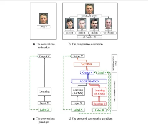
In the literature, the conventional way for facial age esti-mation is a direct method to estimate the age of a person by analysing his/her facial information (e.g., eyes, nose and so forth) directly from the facial image of the person, cf. Fig. 1a, c. In particular, only the input image is taken to estimate the person’s age. However, telling someone’s pre-cise age at a glance without any reference information is essentially difficult even for humans [10]. In responding to the above challenges, our idea is to develop a facial age estimation algorithm inspired by human cognitive pro-cesses [12]. In practice, humans commonly use several judgements to estimate one person’s age, cf. Fig. 1b. First, they learn to establish connections between a known age and the corresponding facial cues of a person (the direct method) and second, they take the learnt knowledge as reference to judge if an unseen face is younger or older than the reference (the comparative method). The larger
Fig. 1Schematic diagram ofa,cthe conventional paradigm for facial age estimation by learning the age information from a facial image directly, and
b,dthe proposed paradigm by aggregating the comparisons of a facial image with baseline samples to determine the age in a comparative manner
the number of available references are, the more precise the age of an unseen face can be estimated.
Therefore, a general mathematical framework, namely Comparative Region-Convolutional Neural Network (CRCNN), is proposed for facial age estimation, cf. Fig. 1d. Conceptually, we compare an unseen face with a set of selected references (labelled baseline samples) to determine if the person of the unseen face is younger or older than each of the baseline persons. We couple this comparative scheme with a specific deep learning architecture, namely Region-Convolutional Neural Net-work (R-CNN) [13]. The R-CNN is exploited to extract the most “iconic” local region from each facial image, where the spatial context (geometrical interrelation) of the extracted local regions can be also accounted for robust classification. In the proposed CRCNN frame-work, not only the input image is used, but also several
Further, the traditional way to learn the parameters of a deep architecture is to minimize an objective func-tion by computing the gradient over all the parameters using the backpropagation algorithm [14] with a nonlin-ear optimizer. However, the deep lnonlin-earning method has been observed to be very difficult to train especially due to the ill-conditioning problem and local minima issue [15]. These difficulties also complicate the manual tuning of deep learning parameters as well as the convergence. In this work, we propose to incorporate the recent Method of Auxiliary Coordinates (MAC) [16] into our framework for training, which appears to open an interesting door toward more efficient training of deep architecture. The method introduces a set of variables to break the objec-tive function dependency, which makes the problem much better conditioned without nesting, affording an efficient and distributed optimization.
Our main contributions are multifold: first, to the best of our knowledge, our CRCNN framework is the first com-parative deep learning approach for facial age estimation and has demonstrated its outperformance over the state-of-the-art methods by experimenting with well-known face datasets. In addition, instead of using the classical deep learning techniques, e.g., Convolutional Neural Net-work (CNN) [17], we proposed the use of R-CNN to account for the spatial context of facial regions; secondly, we improved the training efficiency of deep architecture by incorporating the MAC techinique. The notorious ill-conditioning problem of deep learning can be alleviated; thirdly, we implemented our mathematical framework with CAFFE [18], a popular deep learning platform which exploits the parallelization over multiple GPUs. The com-patibility with CAFFE makes all the components of our mathematical implementation readily available to be used by other researchers; fourthly, observing the fact that the sensitivity of deep learning parameters makes it a non-trivial task to obtain an appropriate setting, the systematic investigation on parametric optimization provides a guid-ance to users who would extend our approach for their future researches.
This paper is organized as follows. Section 2 describes the related work. Section 3 presents our algorithm, and Section 4 gives experimental results to demonstrate the optimization and the various advantages of our approach. Section 5 draws the conclusions and gives directions for future work.
2 Related work
Many researchers have developed techniques for facial age estimation. Most of the previous works focus on the extraction and fusion of different types of facial features: the extraction of local features by using various meth-ods [9]; the combination of hybrid features (e.g., Gabor filters and local binary patterns) by using hierarchical
classifiers based on support vector machines (SVMs) and support vector regression (SVR) [8, 19]; the fusion of tex-tural and local appearance based descriptors to achieve faster and more accurate results [20]; the use of canonical correlation analysis (CCA) for jointly estimating the age with other facial information like gender [21]. Recently, the deep learning has been applied for facial age estima-tion, e.g., a multilayered neural network is integrated with the adapted retinal sampling mechanism [22]; the con-volutional neural network based methods [23, 24] have been studied as well; a constructive probabilistic neural network based on learning from label distributions was also presented [10]. In summary, the previous works all followed the conventional paradigm, i.e., learning direct mappings between the extracted facial features and the associated age labels. These observations motivated the development of our comparative approach with the deep learning method.
the younger/older comparison will provide robust ranking by leaning similar facial information to estimate similar ranks, thus the ranking will be better structured.
3 The proposed method: a CRCNN framework The proposedComparative Region-Convolutional Neural Network (CRCNN), a general mathematical framework for facial age estimation, is developed by comparing an input face with a number of baseline samples to determine its age. We compare the input face with each baseline sample and determine if the input face is older or younger than the baseline person. A set of hints (comparative relations) is therefore collected. The estimation stage aggregates the set of hints to obtain the age of the input person. In this section, we first explain some preliminary defi-nitions (Section 3.1). Then we give an overview of our CRCNN framework (Section 3.2). Finally each algorith-mic component in our approach is explained in details (Section 3.3).
3.1 Preliminary definitions
Before explaining our CRCNN framework, we first define two terminologies: the baseline and the set of hints.
a) Baseline: The objective is to compare the age of an input image with those of a set of reference images, where the ages of these references are known. We define these references as the baseline. A baseline is composed by a set of reference samples, as many as possible to thoroughly cover the value range of possible ages (e.g., labels). In other words, each baseline sample represents an age label. In a minimum, we take one baseline sample per label, there-fore, if we haveMlabels, then we haveMbaseline samples in total. And if we haveK baseline samples per label, we will have totallyMKbaseline samples.
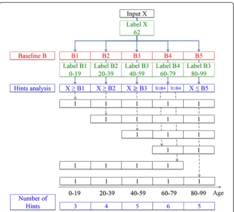
b) Set of hints: To understand the exploitation of the set of hints, we follow the example in Fig. 2. To esti-mate the age of an inputX(the ground-truth age is 62), we first compare the input with the baseline samples
B= {B1,. . .,B5}. A hint can be in two categorical types: “younger” or “older”.1For each baseline sample, if the age of the input is estimated to be larger than the age of the baseline sample (i.e., the input person is estimated to be “older” than the baseline one), we add a hint for the corre-sponding label of every baseline sample with its age larger than (or equal to) the comparing one. For example, we consider the comparison between XandB2. SinceXis older than B2, we thus add a hint for the labels of B2, B3,B4, andB5to indicate that they are all possible labels for X. Similarly, if the input person is estimated to be “younger” than the baseline person, then we add a hint for the corresponding label of every baseline sample with its age smaller than (or equal to) the comparing one. In this
Fig. 2Generation of a set of the hints (for simplicity, five labels are presented)
way, the obtained hints of each label in number is propor-tional to the likelihood that a label is the true label to the input, e.g., in Fig. 2,B4is the most likely label toXandB1 is the most unlikely one.
3.2 An overview of our CRCNN framework
Our CRCNN framework can be decomposed into two main stages, as presented in Fig. 1(d):
3.2.1 The comparative stage (collecting the hints)
After building up a baseline, the input image is com-pared with each of the baseline samples. We use the R-CNN deep architecture to extract facial information from the images and then apply an energy function-based aggregation to generate the comparisons (Section 3.3.1). Therefore, a set of hints is collected. Each hint represents a comparative relation (younger or older) which provides information to compute the estimated age at the next stage.
3.2.2 The estimation stage (voting the hints)
This stage votes by the results from the set of hints to compute the estimated age (Section 3.3.2).
3.3 The CRCNN formulations
ConsideringIas a universal set of facial images andLbe the corresponding label set of possible ages of a human being, we are given a training set ofNfacial imagesX∈I
and its labelY ∈ L. LetFdenotes the deep architecture function. Instead of computingYwith F as usual in the conventional paradigm:
F:I → L
The idea is to introduce a baselineB = {B1,. . .,BM} from I with a composition function and in order to decompose the task into two main parts. Note thatX
andBare usually disjoint. First, in the comparative stage, the comparison ofXand the baselineBwithprovides the set of hintsH(Section 3.3.1). Second, in the estima-tion stage, the vote of hints from the set of hintsHis to obtain the final labelLwith(Section 3.3.2). Therefore, the proposed CRCNN approach is formulated as follows:
(I×I) −→ H −→ L
(X,B) →Z=(X,B) →Y=(Z).
3.3.1 The comparative stage
The set of hintsZ∈His computed fromX∈IandB∈I
with the functionwhich is decomposed into: =R◦C◦L◦F◦A.
The first operatorRdetects all the regions where the facial information is selected by R-CNN to be the most relevant. The second operator C is the convolutional step (including sub-sampling layers) that extracts a fixed-length feature vector from each region. The third and fourth operators (L and F) are the locally and fully-connected steps [17]. Finally, the features of both the input image and baseline samples are aggregated into the last operatorAwhere an energy function approximates the age comparison with a distance metric.
Region-detection layer: Consider Xi ∈ I, an input image, a set of candidate regions{Xi,j}j=1...J is detected fromXiin order to extract more efficient facial informa-tion features. Each regionXi,jis detected by the algorithm in [13]. The same region-detection operatorRis applied to each baseline sampleBm providing a set of candidate regions{Bm,j}j=1...J. Therefore, we denote byH1the first hidden layer of our deep architecture, formed with the region-detection layer. Notice that, if no region detection is used (Ris equivalent to an identical function), then we set the output as the input image itself ({Xi} = {Xi}).
Convolutional layers: The convolutional operator C extracts features from the first hidden layerH1. Specif-ically, features are computed by forward propagating through a convolutional structure of|C|layers with
C=C
1 ◦2C◦ · · · ◦|CC|.
These steps expand the input into a set of simple local features. We denoteHk = kC(Hk−1) as the output of a convolutional layer for k = 2, 3,. . .,|C| + 1. More details of the convolutional layer can be referred to [17]. We interpret these convolutional steps as an adaptive pre-processing step. The purpose of these convolutional steps is to extract low-level features, like simple edges and tex-tures. Notice that the sub-sampling layers make the output
of convolution networks more robust to local transla-tions and small registrational errors, which is important in facial recognition problem.
Locally-connected layers: After extracting features with C, applied independently toX
iandBm, we first combine locally extracted features through |L| locally-connected layers with
L=L
1◦2L◦ · · · ◦|LL|,
resulting to Hk = kL(Hk−1) for k = |C| + 2,|C| + 3,. . .,|C|+|L|+1. Like in the convolutional deep learning, the locally-connected layers apply a filter bank, but every location in the feature map learns a different set of filters. For example, information from an area between the eyes and the eyebrows will be combined with the one between the nose and the mouth, but the two pieces of infor-mation will be processed differently in the convolutional operation.
Fully-connected layers: Then, the fully-connected oper-ationFcomputes all the weights together with
F=F
1 ◦2F◦ · · · ◦|FF|
andHk = kF(Hk−1)fork = |C| + |L| +2,|C| + |L| + 3,. . .,|C| + |L| + |F| +1. Unlike in the locally-connected operation where the inputs are locally combined, each output unit in the fully connected layers is connected to all inputs. These layers are able to capture correla-tions between features captured in distant parts of the face images, e.g., the position and shape of eyes and the position and shape of mouths.
Aggregation: An EBM energy function [28] is exploited to aggregate both information ofXiandBmfrom the fully-connected operation in order to estimate ifXiis younger or older thanBm. The advantage of the adopted energy function is that there is no need for estimating normalized probability distributions over the input space. The scalar energy function E measures the compatibility between
Xi and Bm and leads to a set of hints associated with the in-between comparative relation, cf. Fig. 2. This real-valued energy function is thus defined as E(Xi,Bm) =
||GW(Xi)−GW(Bm)||, where GW is a mapping (subject to learning) to produce output vectors that are nearby for images from the same person, and far away for images from different persons [28].
Learning is then performed by finding the deep archi-tecture parameters that minimize a suitably designed loss function, evaluated over a training set. ConsiderL− (or L+) the partial loss function ifXiis younger (or older) than
Bm, our loss function is of the form
L=1− ¯Zl
L−(E(Xi,Bm))+Z¯l
where Z¯l is the ground truth of the hintZl. The partial loss functionL−(orL+) is designed in such a way that the minimization ofLwill decrease (or increase) the energy when Xis younger (or older) than Bi. A simple way to achieve that is to makeL−monotonically decreasing, and L+monotonically increasing.
3.3.2 The estimation stage
Once the set of hints have been generated, the estimation stage is applied to vote by the output information of the previous comparative stage in order to estimate the per-son’s age. The representation of the set of hints in Fig. 2 includes the number of hints for each label. This result is computed by applying a summation at each label. There-fore, the age of the input person could be estimated by taking the label with the most votes in a naive way. In prac-tice, to avoid the case where the most votes appears in more than one label, we choose to use the real value out-putted from the energy functionEinstead of the number of hintsZi, since the confidence of a vote is also embed-ded. That is, a larger value indicates the higher confidence of a vote, and vice versa.
3.4 Learning method for the comparative stage
In this work, we propose to incorporate the recent Method of Auxiliary Coordinates (MAC) [16] for training the comparative stage. The MAC method decouples the typical learning problem of the comparative stage, which typically has an objective function in the form
minZ− (X,B)2
into the following one:
min Hk+1−k+1(Hk)2 min Z−K(HK)2
fork = 1, 2,. . .,|C| + |L| + |F| andK = |C| + |L| +
|F| +1. Note that the MAC is applied only to the con-volutional, locally- and fully-connected layers, such that k ∈ {kC,kL,kF}. The problem becomes a set of small, independent minimization subproblems, each of which can be easily solved, and without back-propagating any gradients. The objective function is optimized over the hidden layerHand over the weightsW(of the function ) with the two functions below alternatively:
Hk−1
k−1 −→Hk
k
−→Hk+1
Hk k
−→Hk+1
Specifically, optimizing the objective function over the hidden layerHk means optimizing the following nonlin-ear, least-squares regression of the form
min Hk
Hk−k−1(Hk−1)2+ Hk+1−k(Hk)2
and alternatively, optimizing over the weightWk (of the functionk) with
min
Wk Hk+1−k
Wk,Hk
2.
Notice that optimizing over the hidden layer Hk has fixed weightsWkand optimizing over the weightWkhas fixed hidden layerHk. This minimization problem results in several independent, single-layer single-unit problems that can be solved with existing algorithms, without extra programming cost. We solve this nonlinear least-squares fitting problem with a Gauss-Newton approach [29].
4 Experimental results and discussions
In this section, we present the results from a series of experiments designed to optimize and to test the effec-tiveness of our CRCNN framework. We implemented our experiments using CAFFE in a machine with Intel CPU duo-cores (at 3.40 GHz). Firstly, we present the general setting of our experiments. Secondly, we optimize the setting (i.e., try our best to search for the best setting empirically) of our CRCNN approach. Finally, we compare our CRCNN approach with the state-of-the-art methods in facial age estimation.
4.1 Experimental setup
4.1.1 Datasets
4.1.2 Implementation platform
CAFFE [18] is a BSD-licensed C++ library with Python and MATLAB bindings for training and deploying general purpose convolutional neural networks and other deep models efficiently on commodity architectures. It is now a very popular deep learning platform and we chose to implement our CRCNN framework based on it to give high extendibility for future practitioners to integrate their own implementations with our CRCNN framework.
4.1.3 Early and late fusion schemes
We perform our mathematical comparative method with two different schemes: the early fusion and the late fusion [35]. The framework described in this paper first adopts the late fusion scheme, i.e., we extract features from the input image and each baseline sample separately and then fully connect all the information into a final layer of the deep architecture. Alternately, the early fusion scheme
first combines the input image with the baseline sam-ples and then extracts information from the both type of images together in the same time. Both fusion schemes will be optimized, tested, and compared to the state-of-the-art results.
4.2 Optimization of our CRCNN framework
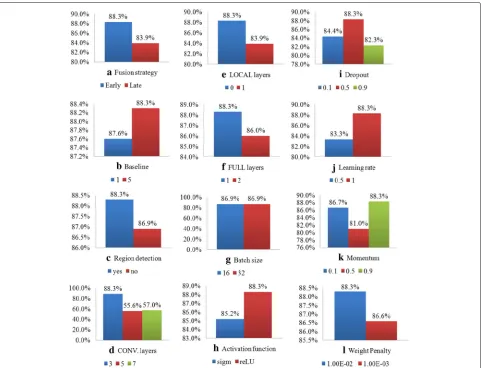
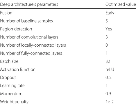
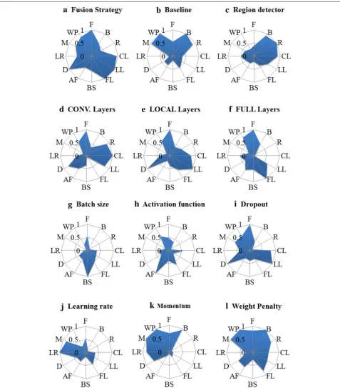
In this section, we present the optimization of our deep architecture. The purpose is to provide insights on the sensitivity of the parameters associated with our CRCNN framework. First, the performance of the comparative stage with different settings of the deep architecture’s parameters (e.g., fusion strategy, baseline, region detec-tion, etc.) is presented in Fig. 3. Each sub-figure repre-sents the performance of a parameter when in different values (or choices). The empirically optimal values of our CRCNN parameters from the experiments are sum-marized in Table 1. Secondly, the sensitivity between
Fig. 3Optimization of our CRCNN approach: performance by different setting of the deep architecture’s parameters.aFusion strategy.bBaseline.
cRegion detection.dCONV. layers.eLOCAL layers.fFULL layers.gBatch size.hActivation function.iDropout.jLearning rate.kMomentum.
Table 1The optimized setting of our CRCNN method
Deep architecture’s parameters Optimized value
Fusion Early
Number of baseline samples 5
Region detection Yes
Number of convolutional layers 3
Number of locally-connected layers 0
Number of fully-connected layers 1
Batch size 32
Activation function reLU
Dropout 0.5
Learning rate 1
Momentum 0.9
Weight penalty 1e-2
parameters is presented in Fig. 4. Each sub-figure repre-sents the correlation coefficient of a parameter and the others based on the obtained performances (of the com-parative stage). The lower the correlation coefficient is (close to 0), the more independent the two parameters are; the higher the correlation coefficient is (close to 1), the more dependency between them on the performance of the comparative stage will be. For example, in Fig. 4g, the correlation coefficient of BS (batch size) and D (dropout) is less than 0.5 (weakly related) and the correlation coeffi-cient of BS and itself is naturally 1 (perfectly related). Note that raw image pixels are taken as the extracted features.
4.2.1 CRCNN parameters:
Fusion strategy (F): The early and the late fusion are dif-ferent in the way of sharing weights. In the early fusion, both types of images (the input one and the baseline ones) share the same set of weights, and in the late fusion, each image has its own weight. As can be seen in Fig. 3a, the first value (88.3%) represents the accuracy when the early fusion is applied to our CRCNN framework, and the sec-ond value (83.9%) represents the accuracy when the late fusion is applied. In other words, Fig. 3a shows a better accuracy when the early fusion is applied. This obser-vation intuitively corresponds to the fact that learning shared weights improves the inner relation between the input image and the baseline. We observe in Fig. 4a that the optimization of each fusion strategy depends on the whole deep architecture (i.e., convolutional layers, locally connected layers, and fully connected layers) and the value of dropout.
Baseline (B): Each baseline sample is taken as a reference to represent a range of possible ages (e.g., labels). In our optimization, we takeMbaseline samples per label, with M = 1, 5. As expected and observed in Fig. 3b, a more
robust computation is provided when M > 1 baseline sample to represent each label. Correlations exist between this parameter and the region detection, and also with sev-eral deep learning parameters, such as the momentum and the weight penalty (Fig. 4b).
Region detection (R): We optimized our method with and without the region detection. In other words, this optimization is equivalent to optimize our CRCNN method by combining the R-CNN [13] or the classical CNN [17]. Figure 3c shows the results of this optimiza-tion and it is clear that region detecoptimiza-tionRcan extract more robust features for improving the performance. The performance of applying this detection depends on the setting of its input (e.g., baseline) and output (e.g., convo-lutional layers) as observed in Fig. 4c.
Convolutional layers (CL): We optimized the convolu-tional layersC relating to the influence of the number of layers. Several numbers of layers have been experi-mented and the results are shown in Fig. 3d. We observe that three convolutional layers provide the best results and the number of layer is logically correlates with its previous and following layers (the region detector and the locally-connected layer C), also with the value of dropout and as mentioned previously, the early/late fusion choice (Fig. 4d).
Locally-connected layers (LL): We optimized the locally-connected layersL. Figure 3e shows the results for different numbers of layers. The most accurate result is provided when the convolutional layer C is directly connected with the fully-connected layerF. Its influence between other parameters is the same as the convolutional layers (Fig. 4e).
Fully-connected layers (FL): The optimization of the fully-connected layersFis shown in Fig. 3f. We observe that only one fully-connected layers is enough to pro-vide the best results. Notice that the optimization of the number of fully connected layer can be set independently (Fig. 4f).
Fig. 4Optimization of our CRCNN approach: sensitivity of the deep architecture’s parameters.aFusion Strategy.bBaseline.cRegion detector.
dCONV. Layers.eLOCAL Layers.fFULL Layers.gBatch size.hActivation function.iDropout.jLearning rate.kMomentum.lWeight Penalty
Activation function (AF): The type of non-linear acti-vation function is typically chosen to be the logistic sig-moid function sigm andreLU. We observe in Fig. 3h that reLU has better accuracy than sigm. Usually, reLUtrains faster and outperforms the other activation
functions. This parameter can be also set independently (Fig. 4h).
a probability such that a hidden unit cannot rely on other hidden units being presented, based on the observation that this parameter is correlating with the deep archi-tecture (Fig. 4i). Previously, we observed the dependency between the influence of this parameter and the early/late fusion choice. Therefore, each fusion strategy leads to its own setting: dropout = 0.5 for the early fusion (Fig. 3i) anddropout = 0for the late fusion.
Learning rate (LR) and momentum (M): We continue the analysis with the learning rate and momentum. Each iteration sees an update of the weight by the computed gradient. The learning rate represents the convergence speed and the momentum parameter introduces a damp-ing effect on the search procedure, thus avoiding oscilla-tions in irregular areas of the error surface by averaging gradient components with opposite signs and accelerat-ing the convergence in long flat areas. In our experi-ments, we observed that in Fig. 3j, k the unit step and the momentum both near to 1 converges better. As a result, we take learning rate = 1and momentum = 0.9, which have to be set dependently (Fig. 4j, k). That is, it has been shown that the use of the momentum in the age estimation task can avoid the search procedure from being stopped in a local minimum and improves the convergence of the back propagation algorithm in general.
Weight penalty (WP): The last parameter is a constraint on the updating weight and we observe in Figs. 3l and 4l that the penalty can be set as penalty = 1e-2 and will influence the setting of several parameters, such as the momentum, the baseline and the fully-connected layers.
In summary, the architecture of our CNN consists of three convolutional layers (CL), each of which is followed by the rectification, max-pooling and normalization. In addition, one fully connected layer (FL) is used. The net-work architecture is detailed as follows:
1. CL: The kernel size is5×5, 1 stride - ReLU - Pool 3×3, 2 stride - Local Response Normalization (LRN). 2. CL: The kernel size is5×5, 1 stride - ReLU - Pool
3×3, 2 stride - Local Response Normalization (LRN). 3. CL: The kernel size is5×5, 1 stride - ReLU - Pool
3×3, 2 stride - Local Response Normalization (LRN). 4. FL.
5. Softmax Loss Layer.
4.2.2 Computational cost
Given an input image, our comparative approach com-pares it with all the k baseline samples, but not with all the N training samples. For example, in our experiments,
each age label is represented by one baseline sample, and totally we have 9 labels, making k = 9. In other words, we only need to compute the comparative relation of the input image for k times, where k can be a small number and much less than N. Therefore, the computational cost of our approach is reasonable.
4.3 Discussions and comparisons with state-of-the-art methods
We compare our approach with others recent facial age estimation techniques such as rKCCA [21], IIS-LLD [10], CPNN [10], OHRank [31], AGES [37] and twoaging func-tion regression based methods, i.e. WAS [38] and AAS [39]. In addition, several conventional general-purpose classification methods,k-Nearest Neighbors (kNN) [40], Back Propagation neural network (BP) [41], C4.5 decision tree [42], Support Vector Machine (SVM) [43], Adaptive Network based Fuzzy Inference System (ANFIS) [44], as well as ranking based approaches are included, such as Ranking SVM [25], RankBoost [26], and RankNet [27]. We trained by using Leave-One-Person-Out (LOPO) test strategy [45], a popular test strategy, as suggested in the related benchmarks [10, 21, 31, 37]. Specifically, we split the used datasets (FG-NET and MORPH) by adopting the same training/testing protocol for all the comparing methods. For example, the LOPO is used on the FG-NET dataset as follows: in each fold, the images of one person are used as the testing set and those of the others are used as the training set. After 82 folds (the FG-NET dataset has a total of 82 subjects), each subject has been used as the testing set in turn, and the average results are computed from all of the estimates. However, since there are more than 13,000 subjects in the MORPH dataset, the LOPO test will be too time-consuming. Thus, we adopted the 10-fold cross validation instead on the MORPH dataset.
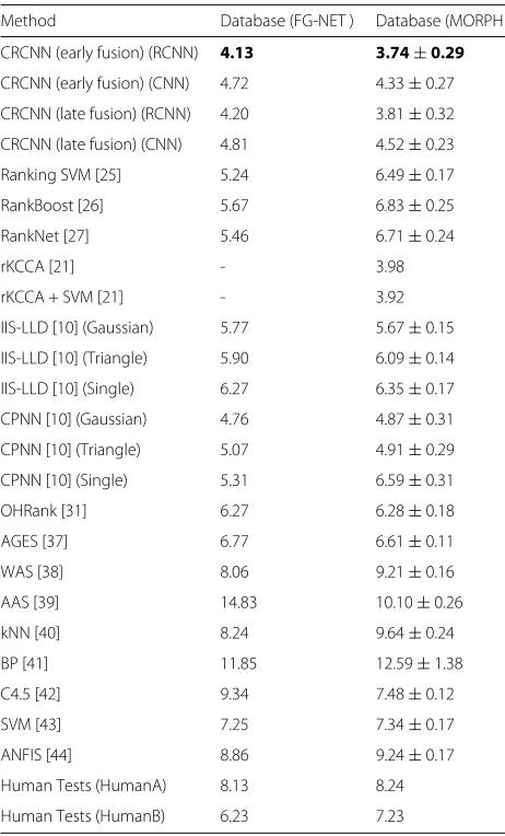
Table 2Comparison with state-of-the-art methods on FG-NET and MORPH databases
Method Database (FG-NET ) Database (MORPH )
CRCNN (early fusion) (RCNN) 4.13 3.74±0.29
CRCNN (early fusion) (CNN) 4.72 4.33±0.27
CRCNN (late fusion) (RCNN) 4.20 3.81±0.32
CRCNN (late fusion) (CNN) 4.81 4.52±0.23
Ranking SVM [25] 5.24 6.49±0.17
RankBoost [26] 5.67 6.83±0.25
RankNet [27] 5.46 6.71±0.24
rKCCA [21] - 3.98
rKCCA + SVM [21] - 3.92
IIS-LLD [10] (Gaussian) 5.77 5.67±0.15
IIS-LLD [10] (Triangle) 5.90 6.09±0.14
IIS-LLD [10] (Single) 6.27 6.35±0.17
CPNN [10] (Gaussian) 4.76 4.87±0.31
CPNN [10] (Triangle) 5.07 4.91±0.29
CPNN [10] (Single) 5.31 6.59±0.31
OHRank [31] 6.27 6.28±0.18
AGES [37] 6.77 6.61±0.11
WAS [38] 8.06 9.21±0.16
AAS [39] 14.83 10.10±0.26
kNN [40] 8.24 9.64±0.24
BP [41] 11.85 12.59±1.38
C4.5 [42] 9.34 7.48±0.12
SVM [43] 7.25 7.34±0.17
ANFIS [44] 8.86 9.24±0.17
Human Tests (HumanA) 8.13 8.24
Human Tests (HumanB) 6.23 7.23
The data in boldface means the best results of FG-NET and MORPH database are both from our CRCNN approach (with the early fusion scheme)
of their papers. For the results of the FG-NET dataset, we follow the common practice of the previous work (e.g., [10]) and do not show the standard deviations. For exam-ple, as mentioned in [10], “the number of images for each person in the FG-NET database varies dramatically. Con-sequently, the standard deviation of the LOPO test on the FG-NET database becomes unstable”. In other words, for the FG-NET database, the values of standard deviation are not so statistically meaningful and thus these values are not shown. The statistics are tabulated in Table 2. As can be seen, the best results (boldfaced) are both from our CRCNN approach (with the early fusion scheme). The second best results are also from our CRCNN approach (with the late fusion scheme). The overall performance of CRCNN is very encouraging. Our results are signif-icantly better than all of the state-of-the-art methods. In comparison to the deep learning based method, i.e. CPNN [10], we also achieved a better performance, with
a relative improvement of 13.24% (from 4.76 to 4.13 on FG-NET) and 23.20% (from 4.87 to 3.74 on MORPH). These facts validate the robustness of the newly proposed comparative approach.
We further performed an evaluation on the IoG database. It consists of 28,231 facial images collected from the Flicker. Each face is labeled in one of the defined seven age groups: 0–2, 3–7, 8–12, 13–19, 20–36, 37–65, and 66+. In our evaluation, we considered only faces having an interocular distance more than 40 pixels, resulting in a subset of 1495 face images. We further reorganized the age labels into the child, teen, and adult classes with the age range of 0–12, 13–19, and 20+, respectively. The set-ting yielded the following amount of samples per each age group: 546, 250, and 699. Finally, we performed the same normalizations as in the previous experiments on all of the IoG faces. We compare our results with the ranking based methods, including [25–27], and Local Binary Pat-tern Kernel Density Estimation (LBP-KDE) [30]. The age group classification performance is represented in Table 3. We can observe better performances of our approach over the state-of-the-art methods, with a relative improvement from 4.74% (in LBP-KDE) to 13.74% (in RankBoost). We believed the outperformance of our CRCNN approach on all the datasets demonstrated its effectiveness for practical applications.
5 Conclusions
This paper proposed a novel comparative deep learning framework for facial age estimation, namely Comparative Region Convolutional Neural Network (CRCNN). Moti-vated by human cognitive processes, we use a comparative approach to determine the age of an unseen person. To the best of our knowledge, it is the first comparative approach in deep learning for facial age estimation and the experimental results validate the outperformance of our CRCNN approach over state-of-the-art methods. One of our future work is to further improve the baseline selec-tion, since obtaining an effective baseline is crucial in our
Table 3Comparison with state-of-the-art methods on IoG database
Method Database (IoG)
CRCNN (early fusion) (RCNN) 66.41%
CRCNN (early fusion) (CNN) 63.16%
CRCNN (late fusion) (RCNN) 65.48%
CRCNN (late fusion) (CNN) 62.19%
LBP-KDE [30] 61.67%
Ranking SVM [25] 56.17%
RankBoost [26] 52.67%
RankNet [27] 55.08%
comparative approach. As aging procedures are quite dif-ferent from person to person, especially from difdif-ferent social groups, we also plan to build a “baseline bank” (con-stituted by a set of baselines, with each corresponds to a computed group of social consistency), instead of using a single and global baseline. Further research on CRCNN in these directions will be attractive future work.
Endnote
1Note that, in this paper, the comparative relations of
“younger” and “older” are actually defined to be “younger than or equal to” and “older than or equal to”, respectively. The “same age” relation thus exists when the two relations hold simultaneously.
Acknowledgements
The authors extend their appreciation to the Deanship of Scientific Research at King Saud University for funding this work through the research group project No. RGP-049.
Authors’ contributions
FA and TL collected the datasets and carried out the experiments. WC and NY constructed the main ideas of the research. AH and MA took part in the examination of the study. All authors read and approved the final manuscript.
Competing interests
The authors declare that they have no competing interests.
Author details
1Social Networks and Human-Centered Computing Program, Taiwan International Graduate Program, Institute of Information Science (IIS), Academia Sinica, Academia Road, Taipei, 11529, Taiwan.2Research Center for Information Technology Innovation (CITI), Academia Sinica, Academia Road, Taipei, 11529, Taiwan.3Department of Computer Science, National Chengchi University, ZhiNan Road, Taipei, 11605, Taiwan.4Department of Software Engineering, College of Computer and Information Sciences, King Saud University, Riyadh, 11362, Saudi Arabia.
Received: 31 July 2016 Accepted: 2 December 2016
References
1. Microsoft Corp, How-Old.net. (2015). https://how-old.net. Accessed 10 July 2016
2. T-H Tsai, W-C Jhou, W-H Cheng, M-C Hu, I-C Shen, T Lim, K-L
Hua, A Ghoneim, MA Hossain, SC Hidayati, Photo sundial: estimating the time of capture in consumer photos. Neurocomputing.177, 529–542 (2016)
3. C-W You, Y-L Chen, W-H Cheng, Socialcrc: enabling socially-consensual rendezvous coordination by mobile phones. Pervasive Mobile Comput.
25, 67–87 (2016)
4. W-H Cheng, C-W Wang, J-L Wu, Video adaptation for small display based on content recomposition. IEEE Trans. Circ. Sys. Video Technol.17(1), 43–58 (2007)
5. B Wu, W-H Cheng, Y Zhang, T Mei, inProceedings of the ACM International
Conference on Multimedia. Time matters: Multi-scale temporalization of
social media popularity, (2016), pp. 1336–1344
6. B Wu, T Mei, W-H Cheng, Y Zhang, inProceedings of the AAAI Conference on Artificial Intelligence. Unfolding temporal dynamics: Predicting social media popularity using multi-scale temporal decomposition, (2016), pp. 272-278
7. Y Fu, G Guo, TS Huang, Age synthesis and estimation via faces: a survey. IEEE Trans. Pattern Anal. Mach. Intell.32(11), 1955–1976 (2010) 8. SE Choi, YJ Lee, SJ Lee, KR Park, J Kim, Age estimation using a hierarchical
classifier based on global and local facial features. J. Pattern Recognit.
44(6), 1262–1281 (2011)
9. SE Choi, YJ Lee, SJ Lee, KR Park, J Kim, inControl Automation Robotics and
Vision (ICARCV), 2010 11th International Conference on. A comparative study
of local feature extraction for age estimation (IEEE, 2010), pp. 1280–1284 10. X Geng, C Yin, Z-H Zhou, Facial age estimation by learning from label
distributions. IEEE Trans. Pattern Anal. Mach. Intell.35(10), 2401–2412 (2013)
11. T Lim, K-L Hua, H-C Wang, K-W Zhao, M-C Hu, W-H Cheng, inProceedings
of the IEEE International Workshop on Multimedia Signal Processing. Vrank:
Voting system on ranking model for human age estimation, (2015), pp. 1–6
12. JB Carroll,Human cognitive abilities: A survey of factor-analytic studies. (Cambridge University Press, New York, 1993)
13. R Girshick, J Donahue, T Darrell, J Malik, Rich feature hierarchies for accurate object detection and semantic segmentation. IEEE Conf. Comput. Vis. Pattern Recognit, 580–587 (2014)
14. T Serre, L Wolf, S Bileschi, M Riesenhuber, T Poggio, Robust object recognition with cortex-like mechanisms. IEEE Trans. Pattern Anal. Mach. Intell.29(3), 411–426 (2007)
15. Y Bengio, inInternational Conference on Statistical Language and Speech
Processing. Deep learning of representations: Looking forward (Springer
Berlin Heidelberg, 2013), pp. 1–37
16. MA Carreira-Perpinan, W Wang, Distributed optimization of deeply nested systems. Int. Conf. Artif. Intell. Stat.33, 10–19 (2014) 17. A Krizhevsky, I Sutskever, G Hinton, Imagenet classification with deep
convolutional neural networks. Conf. Neural Inf. Process. Syst, 1097–1105 (2012)
18. Y Jia, E Shelhamer, J Donahue, S Karayev, J Long, R Girshick, S Guadarrama, T Darrell, inProceedings of the 22nd ACM international conference on
Multimedia. Caffe: Convolutional architecture for fast feature embedding
(ACM, 2014), pp. 675–678
19. JK Pontes, AS Britto, C Fookes, AL Koerich, A flexible hierarchical approach for facial age estimation based on multiple features. Pattern Recognit.54, 34–51 (2016)
20. I Huerta, C Fernandez, A Prati, Facial age estimation through the fusion of texture and local appearance descriptors. Eur. Conf. Comput. Vis. Workshop, 667–681 (2014)
21. G Guo, G Mu, A framework for joint estimation of age, gender and ethnicity on a large database. Image Vis. Comput.32(10), 761–770 (2014) 22. H Takimoto, Y Mitsukura, M Fukumi, N Akamatsu, Robust gender and age estimation under varying facial pose. Electronics Commun. Japan.91(7), 32–40 (2008)
23. C Yan, C Lang, T Wang, X Du, C Zhang, Age estimation based on convolutional neural network. Adv. Multimedia Inf. Process.8879, 211–220 (2014)
24. F Gurpinar, H Kaya, H Dibeklioglu, A Salah, inProceedings of the IEEE
Conference on Computer Vision and Pattern Recognition Workshops. Kernel
elm and cnn based facial age estimation, (2016), pp. 80–86 25. T Joachims, Optimizing search engines using clickthrough data.
International Conference on Knowledge Discovery and Data Mining, 133–142 (2002)
26. Y Freund, R Iyer, RE Schapire, Y Singer, An efficient boosting algorithm for combining preferences. Journal of Machine Learning Research, 4(Nov), 933-969 (2003)
27. C Burges, T Shaked, E Renshaw, A Lazier, M Deeds, N Hamilton, G Hullender, Learning to rank using gradient descent. International Conference on Machine Learning, 89-96 (2005)
28. S Chopra, R Hadsell, Y LeCun, Learning a similarity metric discriminatively, with application to face verification. IEEE Conf. Comput. Vis. Pattern Recognit.1, 539–546 (2005)
29. J Nocedal, SJ Wright, Numerical optimization. Springer Series in Operations Research and Financial Engineering (2006)
30. J Ylioinas, A Hadid, X Hong, M Pietikäinen, Age estimation using local binary pattern kernel density estimate. Int. Conf. Image Anal. Process.
8156, 141–150 (2013)
31. K-Y Chang, C-S Chen, Y-P Hung, inComputer Vision and Pattern
Recognition (CVPR), 2011 IEEE Conference on. Ordinal hyperplanes ranker
with cost sensitivities for age estimation, (2011), pp. 585–592 32. A Lanitis, CJ Taylor, T Cootes, Toward automatic simulation of aging
33. K Ricanek, T Tesafaye, Morph: a longitudinal image database of normal adult age-progression. International Conference on Automatic Face and Gesture Recognition, 341–345 (2006)
34. AC Gallagher, T Chen, Using group prior to identify people in consumer images. IEEE Conference on Computer Vision and Pattern Recognition, 1-8 (2007)
35. J Sanchez-Riera, K-L Hua, Y-S Hsiao, T Lim, SC Hidayati, W-H Cheng, A comparative study of data fusion for rgb-d based visual recognition. Pattern Recognit. Lett.73, 1–6 (2016)
36. M Li, T Zhang, Y Chen, A Smola, inProceedings of the 20th ACM SIGKDD
international conference on Knowledge discovery and data mining. Efficient
mini-batch training for stochastic optimization, (2014), pp. 661–670 37. X Geng, W-H Zhou, K Smith-Miles, Automatic age estimation based on
facial aging patterns. IEEE Trans. Pattern Anal. Mach. Intell.29(12), 2234–2240 (2007)
38. A Lanitis, CJ Taylor, T Cootes, Toward automatic simulation of aging effects on face images. IEEE Trans. Pattern Anal. Mach. Intell.24(4), 442–455 (2002)
39. A Lanitis, C Draganova, C Christodoulou, Comparing different classifiers for automatic age estimation. IEEE Trans. Syst. Man Cybernet.34(1), 621–628 (2004)
40. EA Patrick, FP Fischer, A generalized k-nearest neighbor rule. Inf. Control.
16(2), 128–152 (1970)
41. DE Rumelhart, GE Hinton, RJ Williams, Learning representations by backpropagating errors. Nature.323(9), 533–536 (1986)
42. JR Quinlan,C4.5: Programs for machine learning. (Morgan Kaufmann, San Francisco, 1993)
43. V Vapnik,Statistical learning theory. (Wiley, New York, 1998)
44. R Jang, Anfis: Adaptive network based fuzzy inference system. IEEE Trans. Syst. Man Cybernet.23(3), 665–685 (1993)
45. X Geng, Z-H Zhou, K Smith-Miles, Automatic age estimation based on facial aging patterns. IEEE Trans. Pattern Anal. Mach. Intell.29(12), 2234–2240 (2007)
Submit your manuscript to a
journal and benefi t from:
7Convenient online submission 7Rigorous peer review
7Immediate publication on acceptance 7Open access: articles freely available online 7High visibility within the fi eld
7Retaining the copyright to your article