R E S E A R C H
Open Access
Improved gradient local ternary patterns
for facial expression recognition
Ross P. Holder and Jules R. Tapamo
*Abstract
Automated human emotion detection is a topic of significant interest in the field of computer vision. Over the past decade, much emphasis has been on using facial expression recognition (FER) to extract emotion from facial expressions. Many popular appearance-based methods such as local binary pattern (LBP), local directional pattern (LDP) and local ternary pattern (LTP) have been proposed for this task and have been proven both accurate and efficient. In recent years, much work has been undertaken into improving these methods. The gradient local ternary pattern (GLTP) is one such method aimed at increasing robustness to varying illumination and random noise in the environment. In this paper, GLTP is investigated in more detail and further improvements such as the use of enhanced pre-processing, a more accurate Scharr gradient operator, dimensionality reduction via principal component analysis (PCA) and facial component extraction are proposed. The proposed method was extensively tested on the CK+ and JAFFE datasets using a support vector machine (SVM) and shown to further improve the accuracy and efficiency of GLTP compared to other common and state-of-the-art methods in literature.
Keywords: Facial expression recognition, Gradient local ternary pattern, Scharr operator, Dimensionality reduction, Principal component analysis, Facial component extraction, Support vector machine
1 Introduction
Over the past decade, automated human emotion detec-tion has been a topic of significant interest in the field of computer vision. Two of the most common meth-ods of emotion detection are human behaviour analy-sis [1, 2] and facial expression recognition (FER) [3–5]. In behaviour analysis, an individual’s emotion is deter-mined by analysing their stance and movement patterns, while in FER, emotion is determined from the individual’s facial expression. FER is arguably more descriptive than behaviour analysis [3], and an individual’s face is also less likely to be obscured in crowded areas. Much work has been carried out over the past decade into creating and improving high accuracy, robust methods of FER.
FER consists mainly of three important steps [3]: (1) face detection, (2) facial feature extraction and finally (3) expression classification. In the first step, faces are identi-fied and extracted from the background. Different regions of the face can then be extracted such as the eyebrows, eyes, nose and mouth. The Viola and Jones face detection
*Correspondence: [email protected]
School of Engineering, University of KwaZulu-Natal, Durban 4041, South Africa
algorithm [6, 7] is widely used due to its efficiency, robust-ness and accuracy at identifying faces in uncontrolled backgrounds. Other methods include the use of active shape models (ASM) [8–10] to identify facial points and edges.
In the second step, suitable features that are able to describe the emotion of the face are extracted. The fea-tures are grouped into two main categories: appearance and geometric. In appearance-based methods, an image filter is applied to the whole face or specific facial regions to extract changes in texture due to specific emotions, such as wrinkles and bulges. Common appearance-based feature extraction methods include the use of local binary patterns (LBP) [9, 11–13], local directional patterns (LDP) [12, 14], local ternary patterns (LTP) [15] and Gabor wavelet transform (GWT) [12, 16]. While LBP, which uses grey-level intensity values to encode the texture of an image, is computationally efficient, it has been shown to perform poorly under the presence of non-monotonic illumination variation and random noise as even a small change in grey-level values can easily change the LBP code [17]. LDP employs a different texture coding scheme to that of LBP, where directional edge response values are
used instead of grey-level intensity values. While LDP has been shown to outperform LBP, it tends to produce incon-sistent patterns in uniform and near-uniform regions due to its two-level discrimination coding scheme, and is heav-ily dependent on the number of prominent edge direction parameters [18]. To solve this limitation, LTP, which adds an extra discrimination level and uses ternary codes as opposed to binary codes in LBP, was introduced. More recently, the gradient local ternary pattern (GLTP) [19] method has been proposed which combines advantages of the previous methods. GLTP uses a three-level dis-crimination ternary coding scheme of gradient magnitude values to encode the texture of an image.
Geometric methods focus on extracting features that measure the distance between certain points on the face such as the distance between corners of the eye and mouth. The shape of various facial components due to changing emotions can also be extracted. Geometric-based feature extraction is often considered more difficult to implement than appearance-based methods due to the variability in the size and shape of features across emo-tions [3]. In [10], Bezier curves were used to accurately represent the shape of each facial component under dif-ferent expressions using four control points. The distance and angle of the end points were used to describe each emotion. With the advent of 3D imaging systems, meth-ods for 3D FER [20] and more recently 4D FER [21] have also been proposed. Unlike traditional 2D meth-ods of FER, 3D FER classifies emotion by extracting the geometric structure of faces from 3D facial scans. 4D FER exists when temporal information is used to con-vey variations in adjacent 3D facial scans. While 3D/4D FER is still a relatively new concept, results have shown it to be effective at addressing the limitations of illumi-nation and pose variation still present in most 2D FER techniques.
Because of the large amount of data that can be extracted from a face, a significant portion constitutes redundant information. Large feature sets can greatly reduce programme efficiency, especially when training a classifier. Dimensionality reduction (DR) techniques are often used to reduce the size of the feature set by remov-ing redundant data, greatly improvremov-ing efficiency without reducing accuracy. Common dimensionality reduction techniques include principal component analysis (PCA) [7, 14, 22, 23], independent component analysis (ICA) [3], linear discriminant analysis (LDA) [3] and AdaBoost [14, 24]. In [7], a combination of multiple feature sets and PCA was used for FER. It was shown that using multi-ple feature sets resulted in a high classification accuracy. By combining the method with PCA for dimensionality reduction, efficiency was improved to an acceptable level comparable to that of other appearance-based methods. Similarly, in [25], canonical correlation analysis (CCA)
was used to fuse together multiple transform domain feature sets to improve classification accuracy. To reduce the overall size of the feature vector, two-dimensional PCA (2DPCA) [26], a more efficient version of PCA, was used to reduce the size of the feature sets before classification.
Besides the traditional appearance and geometric-based methods, other feature selection methods have also been proposed in recent literature. In [27, 28], a deep belief network (DBN) [29] was used for feature selection, learn-ing and classification. However, the results reported do not show a significant increase in recognition accuracy over traditional methods. In comparison, the computa-tional cost of deep learning is much higher than that of traditional methods. More recently, work has been undertaken into dynamic FER. In contrast to traditional FER methods, dynamic FER aims to determine emotion from a sequence of images as opposed to a single static image. In [30], atlas construction and sparse representa-tion were used to extract spatial and temporal informa-tion from a dynamic expression. By including temporal information along with spatial information, greater recog-nition accuracies were achieved compared to that of static image FER. However, computational cost is also greater with dynamic FER depending on the length of the image sequence.
The third and final step of FER is to create a classifier based on the features extracted in step two. The extracted features are fed into a machine learning algorithm that attempts to classify them into distinct classes of emotion based on the similarities between feature data. Once the classifier has been trained, it is used to assign input fea-tures to a particular class of emotion. It is widely accepted that there are seven universally recognizable emotions, as first proposed by Ekman [31]: joy, surprise, anger, fear, disgust, sadness and neutral emotion. Common super-vised classifiers include support vector machines (SVM) [7, 9, 10, 14, 19, 32], K-nearest neighbours (K-NN) [12, 33] and neural networks (NN) [10, 12, 34] . It has been shown that for the task of FER, SVM with a radial basis function (RBF) kernel [9, 10, 14] out-performs other classifiers including alternative kernel SVMs [10, 12].
The remainder of this paper is organized as follows. In Section 2, the methodology for feature extraction and classification is discussed in detail. The experimental setup is outlined in Section 3. In Section 4, the results are presented and discussed. Finally, Section 5 concludes the paper.
2 Materials and methods
2.1 Gradient local ternary pattern
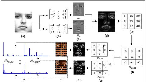
Gradient local ternary pattern (GLTP) is a local appearance-based facial texture feature proposed by Ahmed and Hossain [19]. GLTP is used to encode the local texture of a facial expression by calculating the gradient magnitudes of local neighbourhoods within the image and quantizing the values into three different discrimination levels. The resulting local patterns are used as facial feature descriptors. GLTP aims to address the limitations of common appearance-based features LBP [9, 35] and LDP [14] by combining the advantages of the Sobel-LBP [36] and LTP [16] operators. GLTP uses more robust gradient magnitude values as opposed to grey levels with a three-level encoding scheme to discrim-inate between smooth and highly textured facial regions. This ensures the generation of consistent texture patterns even under the presence of illumination variation and random noise.
Firstly, horizontal and vertical approximations of the derivatives of the source image f(x,y) are obtained by applying the Sobel-Feldman [36, 37] operator. A Sobel operator convolves the source image with horizontal and vertical masks to obtain the horizontal (Gx) and vertical (Gy) approximations of the derivatives respectively (see Fig. 1a–c). The gradient magnitude (Gx,y) (see Fig. 1d) for
each pixel can then be found by combining Gx andGy using the formula:
Gx,y=
G2
x+G2y (1)
Next, to differentiate between smooth and highly textured facial regions, a threshold of±tis applied around a centre gradient value (Gc) of 3×3 pixel neighbourhoods through-out the gradient magnitude image. Neighbour gradient values falling in between Gc+ t and Gc− t are quan-tized to 0, while those below Gc −t and above Gc+t are quantized to−1 and+1 respectively. In other words, we have
SGLTP(Gc,Gi)=
⎧ ⎨ ⎩
−1 Gi<Gc−t
0 Gc−t≤Gi≤Gc+t
+1 Gi>Gc+t
(2)
whereGcis the centre gradient value of a 3×3 neighbour-hood andGi andSGLTP are the gradient magnitude and quantized value of the surrounding neighbours respec-tively (see Fig. 1e, f).
The resulting eight SGLTP values for each 3 × 3 neighbourhood can be concatenated to form a GLTP
(b)
*
*
(c)
(d)
(e)
(a)
(j)
(i)
(h)
(g)
(f)
code. However, using a three-level discrimination coding scheme results in a much higher number of possible pat-terns (38) when compared to that of LBP (28) [9] which would result in a high dimensional feature vector. To reduce the dimensionality, each GLTP code is split into its positive and negative parts and treated as individual codes (see Fig. 1g) as outlined by Tan and Triggs [15]. The for-mula for converting each binary GLTP code to positive (PGLTP) and negative (NGLTP) decimal codes are given in Eqs. 3 and 4.
PGLTP= 7
i=0
SP(SGLTP(i))×2i (3)
SP(v)=
1 ifv>0 0 else
NGLTP = 7
i=0
SN(SGLTP(i))×2i (4)
SN(v)=
1 ifv<0 0 else
After computing the positive (PGLTP) and negative (NGLTP) GLTP decimal coded image representations (see Fig. 1h), each image is divided into m × n regions (see Fig. 1i). A positive (HPGLTP) and negative (HNGLTP)
GLTP histogram is computed for each region using the equations:
HPGLTP(τ)= M m
r=1
N n
c=1
f(PGLTP(r,c),τ) (5)
HNGLTP(τ)= M m
r=1
N n
c=1
f(NGLTP(r,c),τ) (6)
f(α,τ)=
1 ifα=τ 0 else
whereMandNare the width and height, respectively, of the GLTP coded image;randcrepresent row and column, respectively; andτis the GLTP code value (usually, 0–255) for which you are finding the frequency occurrence. By computing a GLTP histogram for each region, the loca-tion informaloca-tion of the GLTP micro-patterns are com-bined with their occurrence frequencies, thus improving recognition accuracy.
Finally, the positive and negative GLTP histogram for each region are concatenated together to form the feature vector (see Fig. 1j) as shown:
HPGLTP(1, 1)HNGLTP(1, 1)
· · ·
HPGLTP(m,n)HNGLTP(m,n)
(7)
Algorithm 1Gradient Local Ternary Pattern
Require: Source image i.e. pre-processed cropped face
Ensure: Vector of GLTP histograms
1: Compute horizontal (Gx) and vertical (Gy) derivative approximations of image using Sobel operator.
2: Compute the gradient magnitude for each pixel of the
imageGx,y=
G2 x+G2y.
3: Apply threshold of ±t around centre gradient value (Gc) in a 3× 3 neighbourhood to determineSGLTP codes for the image.
4: Compute positive (PGLTP) and negative (NGLTP) GLTP coded image representations fromSGLTPvalues.
5: Split coded images intom×nregions.
6: Compute positive (HPGLTP) and negative (HNGLTP) GLTP histogram for each region.
7: Concatenate positive (HPGLTP) and negative (HNGLTP) GLTP histograms from each region to form feature vector.
2.2 Improved gradient local ternary pattern
A common limitation of most appearance-based meth-ods of FER, including GLTP, is that the number of features extracted from images tends to be very large. Unfortunately, most of these features are likely to con-stitute redundant information as not every region of the image is guaranteed to contain the same amount of discriminative data. Having such a large feature set can reduce both the efficiency and accuracy of classi-fication. GLTP also makes use of the inaccurate Sobel operator for computing the gradient magnitude image when more accurate gradient operators could have been used. In this section, improvements to the GLTP method are proposed. These include the use of a more accu-rate Scharr gradient operator, dimensionality reduction to reduce the size of the feature vector, and facial component extraction.
2.2.1 Scharr operator
shown in Fig. 2 [39], and a comparison of Sobel and Scharr gradient magnitude images is given in Fig. 3.
2.2.2 Dimensionality reduction
Having too few features within a feature vector will most often result in classification failure even when using the best of classifiers. On the other hand, having a very large feature vector will make the classification process slow and is not guaranteed to increase classification accuracy. This is especially true if the feature vector contains large amounts of redundant data. To solve this issue, a dimen-sionality reduction (DR) [40] technique is proposed to reduce the size of the feature vector, improving clas-sification efficiency without compromising recognition accuracy. Principal component analysis (PCA) [22] is a technique that is used to transform existing features into a newly reduced set of features. PCA has widely been used for face and expression recognition [23, 41] with good accuracy and more recently has also been used as a DR technique [7, 14, 42, 43]. Using PCA, a covari-ance data matrix is used to compute eigenvectors for a set of data. A linear weighted combination of the top-most few eigenvectors is used to approximate each input feature. All the eigenvectors define the eigenspace, and each eigenvalue defines its corresponding axis of vari-ance. Eigenvalues that are close to zero are discarded as they do not contain much discriminative informa-tion. The eigenvectors associated with the top eigenvalues define the reduced subspace, and the original feature vector can be projected onto this subspace to reduce its size.
2.2.3 Facial component extraction
Each region of a face contains varying amounts of dis-criminative information with regard to facial expres-sion. Regions around the eyes, nose and mouth tend to produce the most discriminative information [44] for appearance-based feature extraction methods. However, many appearance-based FER methods, including GLTP, still populate feature vectors using information obtained from the whole face [9, 14, 19]. This makes the feature vector unnecessarily large by filling it with redundant
(a)
(b)
Fig. 2Scharrahorizontal andbvertical masks for a 3×3 kernel
(a)
(b)
Fig. 3 aSobel gradient magnitude image.bScharr gradient magnitude image
data that contains no discriminative expression informa-tion, such as that from the edges of the face. In certain cases, the subject’s hair or other obscurities that lie at the edge of the face could unintentionally be included as part of the information in the feature vector. This, combined with a large amount of redundant information, could have a potentially negative effect on classification accuracy. Results from literature have shown that performing fea-ture extraction on specific cropped regions of the face can improve classification accuracy [12, 44].
Algorithm 2Improved Gradient Local Ternary Pattern
Require: Source images i.e. pre-processed cropped facial components
Ensure: Feature vector with dimension reduced
1: Compute horizontal (Gx) and vertical (Gy) derivative of each component using Scharr operator.
2: Compute the gradient magnitude for each component
Gx,y=
G2 x+G2y.
3: Apply threshold of ±t around centre gradient value (Gc) in a 3×3 neighbourhood to determine SGLTP codes for each component.
4: For each component, compute positive (PGLTP) and negative (NGLTP) GLTP coded image representations fromSGLTPvalues.
5: Split coded images intom×nregions.
6: Compute positive (HPGLTP) and negative (HNGLTP) GLTP histogram for each region.
7: For each component, concatenate positive(HPGLTP) and negative (HNGLTP) GLTP histograms from each region.
8: Concatenate the extended histograms from each
com-ponent to form feature vector.
2.3 Classification using SVM
A support vector machine (SVM) [32] was used for fea-ture classification. SVM is a supervised machine learning technique that implicitly maps labelled training data into a higher dimensional feature space, constructing a lin-early separable optimal hyperplane between the data. The hyperplane is said to be optimal when the separating mar-gin between the sample classes is maximal. The optimal-hyperplane can then be used to classify new examples. Given a set of labelled training data: T = {(xi,li),i = 1, 2,. . .,L}, wherexi ∈ RP andli ∈ {−1, 1}, a new test samplexis classified by:
f(x)=sign
L
i=1
αiliK(xi,x)+b (8)
whereαiare Lagrange multipliers of the dual optimization problem, K(xi,x) is a kernel function andb is a bias or threshold parameter. The training samples (xi) withαi > 0 are the support vectors. The hyperplane maximizes the margin between these support vectors.
SVM is traditionally a binary classifier that constructs an optimal hyperplane from positive and negative sam-ples. For multi-class classification, the one-against-rest approach was employed. In this approach, a binary clas-sifier is trained for each expression to discriminate one expression from the rest. A radial basis function (RBF) kernel was used for classification. The RBF kernel is defined by the equation:
K(xi,x)=exp
−γ xi−x2
,γ >0 (9)
whereγ is a user selectable kernel parameter.
3 Experimental setup
In this section, an explanation of the datasets used for test-ing and relevant pre-processtest-ing steps are given. Finally, the methods used for parameter selection are detailed.
3.1 Datasets
Two of the most commonly used facial expression datasets in current literature were selected for testing.
3.1.1 CK+ dataset
The Cohn-Kanade (CK) AU-coded expression dataset [45] consists of 97 university students between 18 to 30 years of age. Sixty-five percent were female, 15% were African-American and 3% were Asian or Latino. Subjects were asked to perform up to six different prototypic emo-tions (i.e. joy, surprise, anger, fear, disgust and sadness) as well as a neutral expression. Image sequences from the neutral expression to target expression were captured using a frontal facing camera and digitized to 640×480 or 490 pixels in .png image format.
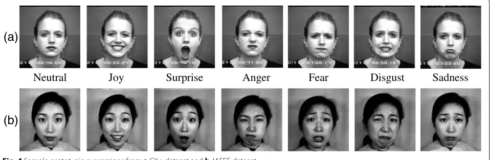
Released in 2010, The extended Cohn-Kanade (CK+) dataset [46] increases the number of subjects from CK by 27% to 123 subjects and the number of image sequences by 22% to 593 sequences. Each peak expression is fully FACS coded and where applicable is assigned a prototypic emotion label. In our setup, 309 sequences were selected from 106 subjects by eliminating sequences that did not belong to one of the six previously mentioned prototypic emotions based on the provided validated emotion labels. For 6-class expression recognition, the three most expres-sive images from each sequence were selected, resulting in 927 images. To build the 7-class dataset, the first image (neutral expression) from each of the 309 sequences was selected and added to the 6-class dataset, resulting in a total of 1236 images. Figure 4a shows a sample of seven prototypic expressions from the CK+ dataset.
3.1.2 JAFFE dataset
The Japanese Female Facial Expression (JAFFE) dataset [47] contains 213 images of 10 female Japanese subjects. Each subject was asked to perform multiple poses of seven basic prototypic expressions. The expression label for each image represents the expression that the subject
Neutral
Joy
Surprise
Anger
Fear
Disgust Sadness
(a)
(b)
was asked to pose. The images are provided in .tiff image format with a resolution of 256×256 pixels. Figure 4b shows a sample of seven prototypic expressions from the JAFFE dataset.
3.2 Pre-processing
To ensure accurate results, the images were pre-processed before feature extraction. Two forms of pre-processing were implemented: cropping the face from the image and cropping multiple facial components from the image.
3.2.1 Cropped face
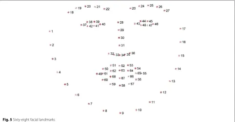
To remove the background and other edge-lying obscuri-ties, the subject’s face was cropped from the original image based on the positions of the eyes. For the CK+ dataset, 68 landmark locations were provided for each image, each of which represents a point on the face as shown in Fig. 5 [11]. Using the provided landmarks, the centres of the left and the right eye were found and the distance (D) between them was calculated. The face was then cropped using empirically selected percentages ofDwith the centre of the left eye as a reference point as shown in Fig. 6. In our setup, the cropping region was reduced to exclude all non-discriminative regions of the face, compared to [14, 19]. After cropping, the faces were resized to a uniform size of 147×108 pixels.
For the JAFFE dataset, no landmark locations are pro-vided. Instead, the popular Viola and Jones [6] face and eye detection cascade was used to detect the face and then the eye location of each image. The face was then cropped
using empirically selected percentages of the width of the detected eyes (W) with the top left corner of the eye region as the reference point as shown in Fig. 7. After cropping, the faces were resized to a uniform size of 147×108 pixels.
3.2.2 Cropped facial components
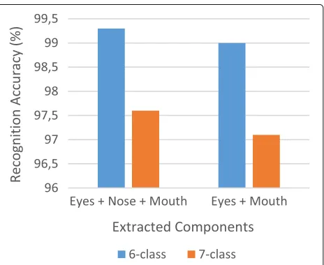
In [7], cropping was performed on the eyes, nose and mouth regions. However, in [12], cropping was only per-formed on the eye and mouth regions with the nose being excluded. In our testing, greater recognition accu-racy was achieved with the mouth region included (see Fig. 9). For the CK+ dataset, the 68 landmark locations (Fig. 5) provided with each image were used to crop the left eye, right eye, nose and mouth regions as shown in Fig. 8a. After cropping, each region is resized to a uniform size of 75×120 pixels and segmented into 3×4 regions as shown in Fig. 8b. For the JAFFE dataset, the eye, nose and mouth regions were found using a common face detection cascade [6].
3.3 Parameter selection
In this section, the methods used to find the optimal parameters for image threshold, component region size, dimensionality reduction and classification are detailed.
3.3.1 Threshold and region size
To find the optimal threshold value t, all other parame-ters were held constant and 10-fold cross-validation was
D 0.6D
0.35D
1.7D
Fig. 6Face cropping in CK+ dataset
performed for increasing values oft. The threshold value that achieved the highest cross-validation accuracy was selected. Thresholds oft=10 andt=20 were confirmed to be the optimal values for the CK+ [19] and JAFFE datasets respectively.
Before extracting GLTP histograms from the face, it is first segmented into m × n regions. This ensures that location information is included together with frequency occurrence information. Having few regions improves classification performance; however, this may result in a low recognition accuracy. On the other hand, having too many regions reduces classification efficiency and may also lower recognition accuracy due to too much unnec-essary location information being included. It has been shown that a region size of 7 × 6 results in optimal recognition accuracy and efficiency [12, 19].
The technique of multiple region segmentation is also used when working with facial components. To deter-mine the optimal region size for each facial component, all parameters are kept constant while varying the region size and performing 10-fold cross-validation. Region sizes of 1×1, 2×2, 2×4, 3×4 and 3×5 were tested. A region size of 3 × 4 resulted in optimal recognition accuracy (see Fig. 10).
3.3.2 Principal component analysis
In principal component analysis (PCA), the number of components selected for projection is a trade-off between
0.2W
W
W
Fig. 7Face cropping in JAFFE dataset
(b)
(a)
Fig. 8 aCropping facial components in the CK+ dataset.b Segmenting each component into a 3×4 region
computational efficiency and recognition accuracy. If too few components remain after applying PCA, efficiency will be high but recognition accuracy will decrease as not enough discriminative features remain in the feature vec-tor. On the other hand, having too large a number of features remaining will not result in any improvement to efficiency. To find the optimal number of principle com-ponents for projection, all parameters were held constant while varying the number of principle components and applying a 10-fold cross-validation test. Projection values of 64, 128, 256, 512 and 1024 were tested, and it was found that the projection value that resulted in optimal accuracy and efficiency was 256 components for the CK+ dataset (see Figs. 11 and 12) and 64 components for the JAFFE dataset.
Fig. 10The effect of varying component region size on recognition accuracy in CK+ dataset
3.3.3 Support vector machine
An optimal parameter grid-search was carried out to find the valuesCandγ using a 10-fold cross-validation testing method as outlined in [32]. The parameter com-bination resulting in the highest cross-validation accuracy was selected.
4 Results and discussion
In this section, results are reported on the CK+ and JAFFE datasets using the methods outlined in Section 2 with a SVM classifier. Finally, comparisons are made between the proposed method and existing methods in literature.
4.1 Testing procedures
Three different testing procedures were used to measure the accuracy of the proposed methodology as outlined in [7, 48]. Details of the procedures are given below.
4.1.1 Cross-validation
Ink-fold cross-validation, the entire dataset is randomly divided into k roughly equally sized segments. In our setup, we usedk= 10 as in [7, 19]. For each fold, 9/10 of the segments are used as the training set while the remain-ing segment is used as the testremain-ing set. This process is
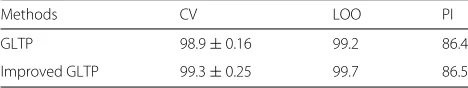
Table 1Recognition rate (%) for 6-class emotion in CK+ dataset using GLTP and Improved GLTP
Methods CV LOO PI
GLTP 98.9±0.16 99.2 86.4
Improved GLTP 99.3±0.25 99.7 86.5
Table 2Recognition rate (%) for 7-class emotion in CK+ dataset using GLTP and Improved GLTP
Methods CV LOO PI
GLTP 96.9±0.21 97.4 83.0
Improved GLTP 97.6±0.30 98.1 83.1
repeated 10 times so that each segment is tested once. The average accuracy is calculated across the 10-folds. Because the dataset is randomly divided, the average accuracy cal-culated will be different each time cross-validation is run. To ensure fair results, 10-fold cross-validation is repeated 10 times and the average overall accuracy is calculated from all 10 runs.
4.1.2 Leave one out
In the leave-one-out method, all images in the dataset apart from one are used as the training set. The remaining image is used for testing. This process is repeated for every image in the dataset so that each image is tested once. The recognition accuracy is found using the equation:
Accuracy= # of correct predictions
total # of images ×100% (10)
4.1.3 Person independent
In the person independent method, all images apart from one subject’s set of expressions are used as the training set (i.e. one subject is completely left out of the training set). The one remaining subject’s images are used as the test set. The process is repeated for each subject. The accuracy from each subject’s test is averaged to obtain the overall accuracy.
4.2 Results on the CK+ dataset
Figure 9 shows a comparison between using four facial components (left eye, right eye, nose and mouth) and three facial components (left eye, right eye and mouth) for feature extraction. Tenfold cross-validation testing was
Table 3Confusion matrix (%) of cross-validation testing method for 6-class emotion in CK+ dataset using Improved GLTP
Joy Sur Ang Fear Dis Sad
Joy 99.9 0 0.1 0 0 0
Sur 0 99.4 0.4 0.1 0 0.1
Ang 0 0 99.3 0 0.4 0.3
Fear 0 0.5 0 99.4 0 0.1
Dis 0 0 0.6 0 99.4 0
Table 4Confusion matrix (%) of cross-validation testing method for 7-class emotion in CK+ dataset using Improved GLTP
Joy Sur Ang Fear Dis Sad Neu
Joy 100 0 0 0 0 0 0
Sur 0.5 98 0 0 0 0 1.5
Ang 0 0.1 95.3 0 0 0 4.6
Fear 0 0.4 0 99.2 0 0 0.4
Dis 0 0 0.5 0 98.6 0 0.9
Sad 0 0 0.9 0.4 0 93.9 4.8
Neu 0.1 0 1.8 0.1 0.5 0.9 96.6
performed for six and seven classes of emotion on the CK+ dataset. The results show that higher recognition accuracies are achieved when using four facial compo-nents for feature extraction, i.e. when the nose is included. To determine the optimal number of regions for each component, 10-fold cross-validation was performed for six and seven classes of emotion on the CK+ dataset while varying the region size. The results are shown in Fig. 10. It can be seen that the optimal region size is 3×4. Fur-ther increasing the region size past 3×4 regions does not result in improved recognition accuracy as unnecessarily large amounts of redundant information get incorporated into the feature vector degrading accuracy.
Tables 1 and 2 summarize the recognition rate of GLTP and our proposed method, Improved GLTP, for six and seven classes of emotion in the CK+ dataset. We observe that our proposed method outperforms traditional GLTP by 0.4 to 0.7% in cross-validation testing and 0.5 to 0.7% in leave-one-out testing for six and seven classes of emo-tion respectively. The results for person independent test-ing also show a slight improvement. The results confirm that the proposed enhancements to GLTP such as the use of the more accurate Scharr operator, dimensionality reduction via PCA and facial component extraction, when combined, further improve the recognition accuracy of GLTP.
Table 5Confusion matrix (%) of leave-one-out testing method for 6-class emotion in CK+ dataset using Improved GLTP
Joy Sur Ang Fear Dis Sad
Joy 100 0 0 0 0 0
Sur 0 99.6 0.4 0 0 0
Ang 0 0 100 0 0.4 0.3
Fear 0 0.5 0 100 0 0.1
Dis 0 0 0.6 0 100 0
Sad 0 0 2.4 0 0 97.6
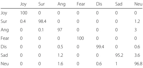
Table 6Confusion matrix (%) of leave-one-out testing method for 7-class emotion in CK+ dataset using Improved GLTP
Joy Sur Ang Fear Dis Sad Neu
Joy 100 0 0 0 0 0 0
Sur 0.4 98.4 0 0 0 0 1.2
Ang 0 0.1 97 0 0 0 3
Fear 0 0 0 100 0 0 0
Dis 0 0 0.5 0 99.4 0 0.6
Sad 0 0 1.2 0 0 95.2 3.6
Neu 0 0 1.6 0 0.6 1 96.8
Tables 3 and 4 show the confusion matrices for 10-fold cross-validation testing for six and seven classes of emotion using Improved GLTP in the CK+ dataset. We observe that, in particular, anger and sadness emotions get confused with neutral emotion in 7-class CV testing.
Tables 5 and 6 show the confusion matrices for leave-one-out testing for six and seven classes of emotion using Improved GLTP in the CK+ dataset. As expected, the leave-out-out testing procedure achieved the highest recognition accuracies on test. This is because, for each fold, the entire dataset apart from one image is used as the training set. Although high accuracies were achieved for both six and seven classes of emotion, we observe that anger and sadness emotions do get confused with the added neutral emotion in 7-class testing, reducing overall accuracy.
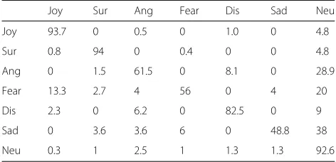
Tables 7 and 8 show the confusion matrices for person independent testing for six and seven classes of emotion using Improved GLTP in the CK+ dataset. This testing procedure achieved the lowest recognition accuracies on test. This is because not a single image from the test subject remains in the training set. Person independent testing is thus used to show the robustness of the method under test to unseen subjects. We observe that in 6-class testing, anger, fear and sadness emotions are misclassi-fied the most. In 7-class testing, the accuracies further
Table 7Confusion matrix (%) of person independent testing method for 6-class emotion in CK+ dataset using Improved GLTP
Joy Sur Ang Fear Dis Sad
Joy 96.6 0 1.9 0 1.5 0
Sur 0.8 97.2 1.2 0.4 0.4 0
Ang 0 4.4 78.5 0 11.9 5.2
Fear 16 6.7 6.7 58.6 0 12
Dis 2.3 0 11.3 0 86.4 0
Table 8Confusion matrix (%) of person independent testing method for 7-class emotion in CK+ dataset using Improved GLTP
Joy Sur Ang Fear Dis Sad Neu
Joy 93.7 0 0.5 0 1.0 0 4.8
Sur 0.8 94 0 0.4 0 0 4.8
Ang 0 1.5 61.5 0 8.1 0 28.9
Fear 13.3 2.7 4 56 0 4 20
Dis 2.3 0 6.2 0 82.5 0 9
Sad 0 3.6 3.6 6 0 48.8 38
Neu 0.3 1 2.5 1 1.3 1.3 92.6
decrease as the emotions also get confused to a great extent with the added neutral emotion.
4.3 Results on the JAFFE dataset
We repeat the cross-validation and leave-one-out tests from above on the JAFFE dataset. The results are summarized in Tables 9 and 10. We see that our proposed method, Improved GLTP, shows a significant improve-ment in recognition accuracy over traditional GLTP for the JAFFE dataset. The largest improvement in recog-nition accuracy was seen during 7-class cross-validation testing, where Improved GLTP outperformed GLTP by 7.3%. Improved GLTP also showed a sizeable improve-ment of 7, 6.3 and 5.5% for 7-class LOO, 6-class CV and 6-class LOO tests respectively. The results from the JAFFE dataset further verifies that the recognition accuracy of Improved GLTP is superior to that of traditional GLTP.
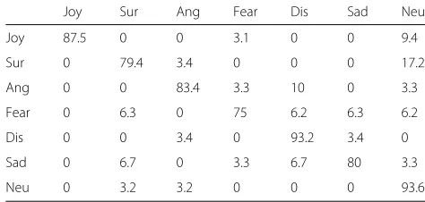
The confusion matrices for cross-validation and leave-one-out tests on the JAFFE dataset are provided in Tables 11, 12, 13 and 14. We observe that, like with the CK+ dataset, leave-one-out testing outperformed cross-validation testing while 7-class testing produced lower recognition accuracies compared to 6-class testing due to the added confusion caused by the included neutral emotion. We also observe that the disgust emotion is the only emotion to not be confused with neutral emotion in 7-class testing.
4.4 Effect of dimensionality reduction
Before performing dimensionality reduction via PCA, it is extremely important to find the optimal number of
Table 9Recognition rate (%) for 6-class emotion in JAFFE dataset using GLTP and Improved GLTP
Methods CV LOO
GLTP 77.0±1.1 81.3
Improved GLTP 83.3±1.6 86.8
Table 10Recognition rate (%) for 7-class emotion in JAFFE dataset using GLTP and Improved GLTP
Methods CV LOO
GLTP 74.4±1.3 77.5
Improved GLTP 81.7±1.3 84.5
components to project. If too many components are set to remain, the time taken to project the increased num-ber of components will outweigh the efficiency improve-ment gained from training/testing the reduced feature set and efficiency will instead decrease. Figures 11 and 12 demonstrate the effect of varying the number of principle components on recognition accuracy and training/testing runtime using 10-fold cross-validation for six and seven classes of emotion in the CK+ dataset. The improvement in runtime is in relation to running Improved GLTP with-out PCA. The results show that projecting a small number of principle components, such as 64, results in a large decrease in runtime but a comparatively lower recognition accuracy. On the other hand, projecting a larger number of principle components, such as 1024, actually increases runtime while recognition accuracy decreases as a result of redundant data being included. It can be seen that the optimal number of principle components to be used for projection is 256.
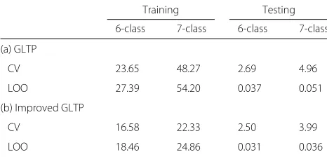
We compare the performance of GLTP to Improved GLTP by comparing the runtime of the training and test-ing stages for 10-fold cross-validation and leave-one-out procedures. We do not consider the person independent procedure as the size of the training and test segments varies per fold. The average per fold runtime for each method using the CK+ dataset is given in Table 15 (Core 2 Duo, 2.0 GHz, 3-GB RAM). The improvement in runtime when using Improved GLTP is shown in Table 16, and the overall improvement in runtime across all folds is given in Table 17.
The results show that Improved GLTP, with dimension-ality reduction via PCA, had a positive effect on runtime
Table 11Confusion matrix (%) of cross-validation testing method for 6-class emotion in JAFFE dataset using Improved GLTP
Joy Sur Ang Fear Dis Sad
Joy 89.1 0.3 0 3.1 0.6 6.9
Sur 3.4 84.5 4.1 5.2 0.7 2.1
Ang 0 1.3 81.7 6 9.3 1.7
Fear 3.1 7.5 0.9 75.4 5 8.1
Dis 0 0 5.5 1.4 89 4.1
Table 12Confusion matrix (%) of cross-validation testing method for 7-class emotion in JAFFE dataset using Improved GLTP
Joy Sur Ang Fear Dis Sad Neu
Joy 86.9 0 0 3.4 0 0.3 9.4
Sur 0 76.6 3.1 1.7 0.7 0 17.9
Ang 0 2.3 78.4 4.7 10.3 0.3 4
Fear 1.3 5.9 0.3 74.1 4.1 6.9 7.4
Dis 0 0 4.1 1.4 90.4 4.1 0
Sad 0 5 1 8.6 8 73.7 3.7
Neu 0 3.2 4.5 0 0 0.3 92
performance in the CK+ dataset. The largest improve-ment in runtime was seen during the training stages. In particular, for the leave-one-out procedure, Improved GLTP saved a total of 10.07 h for 7-class training, reducing the overall training runtime by 54.1% compared to GLTP.
We also compare the performance of Improved GLTP to GLTP using the JAFFE dataset. The overall improve-ment in runtime across all folds when using Improved GLTP is given in Table 18. We confirm that Improved GLTP showed an improvement in runtime across all test-ing procedures. Once again, the largest improvement was seen during the training stages. From the results obtained using both datasets, we have verified that Improved GLTP is more efficient than traditional GLTP.
4.5 Comparison to results in literature
Table 19 shows a comparison between common appearance-based methods of FER and other state-of-the-art methods in current literature on the CK dataset. To make a fair and accurate comparison, the results for LBP, LDP, LTP and GLTP are taken from [19] where the exper-imental setup and testing procedure was kept constant for all methods. In [19], a 10-fold cross-validation testing procedure was used on six and seven classes of emotion in the CK dataset. The results confirm that LBP was the least accurate method on test. LDP and LTP outperformed
Table 13Confusion matrix (%) of leave-one-out testing method for 6-class emotion in JAFFE dataset using Improved GLTP
Joy Sur Ang Fear Dis Sad
Joy 90.6 0 0 3.1 0 6.3
Sur 3.4 89.8 3.4 3.4 0 0
Ang 0 0 86.7 3.3 10 0
Fear 0 9.3 0 78.1 6.3 6.3
Dis 0 0 3.4 0 93.2 3.4
Sad 0 6.7 0 3.3 6.7 83.3
Table 14Confusion matrix (%) of leave-one-out testing method for 7-class emotion in JAFFE dataset using Improved GLTP
Joy Sur Ang Fear Dis Sad Neu
Joy 87.5 0 0 3.1 0 0 9.4
Sur 0 79.4 3.4 0 0 0 17.2
Ang 0 0 83.4 3.3 10 0 3.3
Fear 0 6.3 0 75 6.2 6.3 6.2
Dis 0 0 3.4 0 93.2 3.4 0
Sad 0 6.7 0 3.3 6.7 80 3.3
Neu 0 3.2 3.2 0 0 0 93.6
LBP, achieving very similar results to one another with only a 0.1 to 0.5% difference in recognition accuracy. GLTP was the best performing appearance-based method with a 2.8 to 3.5% improvement in recognition accuracy over LDP and LTP. In our testing, we achieved a 98.9 and 96.9% recognition accuracy for 6- and 7-class emotion, respectively, when using GLTP with the same testing procedure. The increase in base method results by 1.7 and 5.2%, respectively, is possibly due to two different reasons. Firstly, our experimental setup differs to [19] in the fact that we selected only the images in the dataset that exhibited a definitive prototypic emotion. Our selec-tion of total images is thus 24% less than in [19]. However, we included 11% more subjects from the extended CK+ dataset to increase variety compared to [19]. Secondly, we refined the pre-processing of the images by further reduc-ing the area of the cropped face. This eliminated much of the redundant areas that remained after pre-processing
Fig. 12The effect of varying the number of projected principle components on recognition accuracy and runtime for seven classes of emotion in the CK+ dataset
in [19]. The combination of including only images with definitive prototypic emotion and a refined method of pre-processing is the likely cause of the increase in the base recognition accuracy of GLTP.
Besides common appearance-based methods, our results are also compared to other state-of-the-art meth-ods in literature. In [27], a deep belief network (DBN) was used for feature extraction and classification. A recognition rate of 91.1% was achieved for seven classes of emotion using a sevenfold cross-validation testing scheme. Then in [28], the method was improved by using a boosted DBN (BDBN). In this method, a recognition accuracy of 96.7% was achieved for six classes of emotion using an eightfold cross-validation testing scheme. If we were to disregard any differences due to the fold size, the results are respectively 6.5 and 2.6% less accurate than our equivalent methods. The computational cost
Table 15Average Runtime per fold (seconds) using CK+ dataset
Training Testing
6-class 7-class 6-class 7-class
(a) GLTP
CV 23.65 48.27 2.69 4.96
LOO 27.39 54.20 0.037 0.051
(b) Improved GLTP
CV 16.58 22.33 2.50 3.99
LOO 18.46 24.86 0.031 0.036
Table 16Improvement in runtime when using Improved GLTP on CK+ dataset
Training Testing
6-class 7-class 6-class 7-class
(a) Per fold improvement (seconds)
CV 7.07 25.94 0.19 0.97
LOO 8.93 29.34 0.006 0.015
(b) Percentage improvement (%)
CV 29.9 53.7 7.1 19.6
LOO 32.6 54.1 16.2 29.4
of deep learning methods is also much greater than our method. In [30], a state-of-the-art method of dynamic FER using atlas construction and sparse representation was presented. A recognition accuracy of 97.2% was achieved for seven classes of emotion using a person independent testing scheme. In our tests, we obtained an 83.1% recognition accuracy when using Improved GLTP with the same testing procedure. The results from the two methods differ by 14.1% when temporal information is available. However, in [30], the same test was also performed without any temporal information, i.e. only spatial information was used for feature selection. In this case, a recognition accuracy of 92.4% was achieved, 4.8% lower than when temporal information was included. Even without temporal information, the method still achieves a 9.3% higher recognition accuracy than that of Improved GLTP. The results show that dynamic FER can offer much higher recognition accuracies than traditional static methods of FER. However, the compu-tational cost and complexity of working with dynamic image sequences is much greater than when working with static images. The authors report that it takes 1.6 s to predict one image sequence (4-core, 2.5 GHz, 6-GB RAM). In comparison, we found that our proposed method, Improved GLTP, took an average time of under
Table 17Overall improvement in runtime when using Improved GLTP on CK+ dataset
Training Testing
6-class 7-class 6-class 7-class
(a) Seconds
CV 70.7 259.4 1.9 9.7
LOO 8278.1 36264.2 5.6 18.5
(b) Hours
CV 0.0196 0.0721 0.0005 0.0027
Table 18Overall improvement in runtime when using Improved GLTP on JAFFE dataset
Training Testing
6-class 7-class 6-class 7-class
(a) Seconds
CV 11.4 17.6 0.4 0.7
LOO 262.6 535.3 0.7 0.6
(b) Percentage (%)
CV 60.0 66.8 24.2 33.0
LOO 63.5 72.0 30.8 23.1
40 ms for each image prediction (2-core, 2.0 GHz, 3-GB RAM), far less than that of the dynamic-based method. The results are summarized in Fig. 13 where it is shown that our proposed Improved GLTP method outperforms common appearance-based feature extraction methods as well as other state-of-the-art methods in current literature.
5 Conclusions
In this paper, we have confirmed, via extensive test-ing on the CK+ and JAFFE datasets, that gradient local ternary pattern (GLTP) [19] is an accurate and effi-cient feature extraction technique well suited for the task of facial expression recognition (FER). Improvements to GLTP such as the use of enhanced pre-processing, a more accurate Scharr gradient operator, dimension-ality reduction via PCA and facial component extrac-tion were proposed. The Improved GLTP method was implemented and tested and shown to further improve recognition accuracy and efficiency. In a comparison with techniques from current literature, our improved
Table 19Comparison of recognition rate (%) on CK dataset for various feature selection methods in literature
Methoda 6-class 7-class
LBP [18] 90.1 83.3
LDP [18] 93.7 88.4
LTP [18] 93.6 88.9
GLTP [18] 97.2 91.7
DBN [24] - 91.1b
BDBN [25] 96.7c
-Dynamic atlas [27] - 97.2d92.4d, e
Improved GLTP 99.3 97.6
a10-fold cross-validation unless otherwise stated b7-fold cross-validation
c8-fold cross-validation dPerson independent eWithout temporal information
Fig. 13Comparison of feature selection methods on CK dataset
method was shown to outperform other state-of-the-art methods in terms of both recognition accuracy and effi-ciency. In the future, Improved GLTP can be combined with multiple feature sets to further improve recognition accuracy.
Acknowledgements
The authors gratefully acknowledge the PRISM/CSIR for funding this research.
Authors’ contributions
JR-T conceptualized the idea for research, contributed to the data analysis, provided editorial input, co-developed and executed the research and participated in the model and algorithm designs. RP-H developed the research, designed and implemented the system, conducted the experiments and carried out the final validation of the system designed; he also drafted the manuscript. Both authors read and approved the final manuscript.
Competing interests
The authors declare that they have no competing interests.
Publisher’s Note
Springer Nature remains neutral with regard to jurisdictional claims in published maps and institutional affiliations.
Received: 19 September 2016 Accepted: 4 June 2017
References
1. S Danafar, A Giusti, J Schmidhuber, Novel kernel-based recognizers of human actions. EURASIP J. Adv. Signal Process.2010(1) (2010) 2. C Yu, X Wang, Human action classification based on combinational
features from video. J. Comput. Inf. Syst.8(12), 5245–5254 (2012) 3. S Mahto, Y Yadav, A survey on various facial expression recognition
techniques. Int. J. Adv. Res. Electr. Electron. Instrum. Eng.3(11), 13028–13031 (2014)
4. S Mishral, A Dhole, A survey on facial expression recognition techniques. Int. J. Sci. Res. (USR).4, 1247–1250 (2015)
5. J Kumari, R Rajesh, K Pooja, Facial expression recognition: a survey. Procedia Comput. Sci.58, 486–491 (2015)
7. A Shaukat, M Aziz, U Akram, inIT Convergence and Security (ICITCS) 2015 5th International Conference on. Facial Expression Recognition Using Multiple Feature Sets (IEEE, Kuala Lumpur, 2015), pp. 1–5
8. TF Cootes, CJ Taylor, DH Cooper, J Graham, Active shape models-their training and application. Comp. Vision Image Underst.61(1), 38–59 (1995) 9. X Wang, X Liu, L Lu, Z Shen, inComputational Science and Engineering
(CSE) 2014 IEEE 17th International Conference on. A new facial expression recognition method based on geometric alignment and LBP features (IEEE, Chengdu, 2014), pp. 1734–1737
10. H Bao, T Ma, inComputer and Information Technology (CIT) 2014 IEEE International Conference on. Feature extraction and facial expression recognition based on Bezier curve (IEEE, 2014), pp. 884–887 11. C Sagonas, G Tzimiropoulos, S Zafeiriou, M Pantic, inComputer Vision
Workshops (ICCVW), 2013 IEEE International Conference on. 300 Faces in-the-Wild Challenge: The first facial landmark localization Challenge (IEEE, Sydney, 2013)
12. P Suja, S Tripathi, Analysis of emotion recognition from facial expressions using spatial and transform domain methods. Int. J. Adv. Intell. Paradigms. 7(1), 57–73 (2015)
13. D Huang, C Shan, M Ardabilian, Y Wang, L Chen, Local binary patterns and its application to facial image analysis: a survey. IEEE Trans. Syst. Man Cybernet. Part C Appl. Rev.41(6), 765–781 (2011)
14. T Jabid, MH Kabir, O Chae, Robust facial expression recognition based on local directional pattern. ETRI J.32(5), 784–794 (2010)
15. X Tan, B Triggs, Enhanced local texture feature sets for face recognition under difficult lighting conditions. IEEE Trans. Image Process.19(6), 1635–1650 (2010)
16. S Bashyal, GK Venayagamoorthy, Recognition of facial expressions using Gabor wavelets and learning vector quantization. Eng. Appl. Artif. Intell. 21(7), 1056–1064 (2008)
17. H Zhou, R Wang, C Wang, A novel extended local-binary-pattern operator for texture analysis. Inf. Sci.178(22), 4314–4325 (2008)
18. F Ahmed, MH Kabir, inConsumer Electronics (ICCE), 2012 IEEE International Conference on. Directional ternary pattern (dtp) for facial expression recognition (IEEE, Las Vegas, 2012)
19. F Ahmed, E Hossain, Automated facial expression recognition using gradient-based ternary texture patterns. Chin. J. Eng.2013, 1–8 (2013) 20. X Yang, D Huang, Y Wang, L Chen, inAutomatic Face and Gesture
Recognition (FG), 2015 11th IEEE International Conference and Workshops on. Automatic 3D Facial Expression Recognition using Geometric Scattering Representation (IEEE, Ljubljana, 2015)
21. Q Zhen, D Huang, Y Wang, L Chen, Muscular movement model based automatic 3D/4D Facial expression recognition.IEEE Trans. Multimedia. 18(7), 1438–1450 (2016)
22. I Jolliffe,Principal component analysis. (Springer-Verlag, New York, 2002) 23. SS Meher, P Maben, inAdvance Computing Conference (IACC), 2014 IEEE
International. Face recognition and facial expression identification using PCA (IEEE, Gurgaon, 2014), pp. 1093-1098
24. Y Freund, RE Schapire, A desicion-theoretic generalization of on-line learning and an application to boosting. J. Comput. Syst. Sci.55(1), 119–139 (1997)
25. EH El-Shazly, MM Abdelwahab, R-I Taniguchi, inSignal-Image Technology & Internet-Based Systems (SITIS), 2015 11th International Conference on. Efficient Facial and Facial Expression Recognition Using Canonical Correlation Analysis for Transform Domain Features Fusion and Classification (IEEE, Bangkok, 2015), pp. 639–644
26. J Yang, D Zhang, AF Frangi, Yang Jy, Two-dimensional PCA: a new approach to appearance-based face representation and recognition. IEEE Trans. Pattern Anal. Mach. Intell.26(1), 131–137 (2004)
27. Y Lv, Z Feng, C Xu, inSmart Computing (SMARTCOMP), 2014 International Conference on. Facial expression recognition via deep learning (IEEE, Hong Kong, 2014), pp. 303-308
28. P Liu, S Han, Z Meng, Y Tong, inComputer Vision and Pattern Recognition (CVPR), 2014 IEEE Conference on. Facial expression recognition via a boosted deep belief network (IEEE, Columbus, 2014), pp. 1805–1812 29. GE Hinton, S Osindero, YW Teh, A fast learning algorithm for deep belief
nets. Neural Comput.18(7), 1527–1554 (2006)
30. Y Guo, G Zhao, M Pietikäinen, Dynamic facial expression recognition with atlas construction and sparse representation. IEEE Trans. Image Process. 25(5), 1977–1992 (2016)
31. P Ekman, Strong evidence for universals in facial expressions: a reply to Russell’s mistaken critique. Psychol. Bull.115(2), 268–287 (1994) 32. CW Hsu, CJ Lin, A comparison of methods for multiclass support vector
machines. IEEE Trans. Neural Netw.13(2), 415–425 (2002) 33. NS Altman, An introduction to kernel and nearest-neighbor
nonparametric regression. Am. Stat.46(3), 175–185 (1992)
34. N Thomas, M Mathew, inComputing, Communication and Applications (ICCCA), 2012 International Conference on. Facial expression recognition system using neural network and MATLAB (IEEE, Dindigul, 2012) 35. T Ojala, M Pietikainen, T Maenpaa, Multiresolution gray-scale and rotation
invariant texture classification with local binary patterns. IEEE Trans. Pattern Anal. Mach. Intell.24(7), 971–987 (2002)
36. S Zhao, Y Gao, B Zhang, inImage Processing, 2008. ICIP 2008. 15th IEEE International Conference on. Sobel-lbp (IEEE, San Diego, 2008), pp. 2144–2147
37. I Sobel, G Feldman, inPattern Classification and Scene Analysis, ed. by R Duda, P Hart. A 3x3 isotropic gradient operator for image processing, presented at a talk at the Stanford Artificial Project (John Wiley & Sons, 1968), pp. 271–272
38. H Scharr, Optimal operators in digital image processing. PhD thesis (2000) 39. Opencv2 series of learning notes 8 (image filtering). http://www.
programering.com/a/MDM3UzNwATk.html. Accessed 28 July 2016 40. CA Kumar, Analysis of unsupervised dimensionality reduction techniques.
Comput. Sci. Inf. Syst.6(2), 217–227 (2009)
41. MA Turk, AP Pentland, inComputer Vision and Pattern Recognition, 1991. Proceedings CVPR’91., IEEE Computer Society Conference on. Face recognition using eigenfaces (IEEE, Maui, 1991), pp. 586–591
42. HB Deng, LW Jin, LX Zhen, JC Huang, A new facial expression recognition method based on Local Gabor filter bank and PCA plus LDA. Int. J. Inf. Technol.11(11), 86–96 (2005)
43. H Ujir, M Spann, inTopics in Medical Image Processing and Computational Vision, ed. by JMRS Tavares, RN Jorge. Facial Expression Recognition Using FAPs-Based 3DMM (Springer Science & Business Media, 2013), pp. 33–47 44. H Mliki, M Hammami, Discriminative regions selection for facial
expression recognition. Int. J. Comput. Sci. Issues (IJCSI).11(5), 50 (2014) 45. T Kanade, JF Cohn, Y Tian, inAutomatic Face and Gesture Recognition, 2000.
Proceedings. Fourth IEEE International Conference on. Comprehensive database for facial expression analysis (IEEE, Grenoble, 2000), pp. 46–53 46. P Lucey, JF Cohn, T Kanade, J Saragih, Z Ambadar, I Matthews, in
Computer Vision and Pattern Recognition Workshops (CVPRW), 2010 IEEE Computer Society Conference on. The extended cohn-kanade dataset (ck+): A complete dataset for action unit and emotion-specified expression (IEEE, San Francisco, 2010), pp. 94–101
47. MJ Lyons, S Akemastu, M Kamachi, J Gyoba, inAutomatic Face and Gesture Recognition, 1998. Proceedings. Third IEEE International Conference on. Coding Facial Expressions with Gabor Wavelets (IEEE, Nara, 1998), pp. 200-205