R E S E A R C H
Open Access
An adaptive decision based interpolation
scheme for the removal of high density salt
and pepper noise in images
Vasanth Kishorebabu
1*, Ganesan Packyanathan
1, Harikrishna Kamatham
1and Vishnu Shankar
2Abstract
An adaptive decision based inverse distance weighted interpolation (DBIDWI) algorithm for the elimination of high-density salt and pepper noise in images is proposed. The pixel is initially checked for salt and pepper noise. If classified as noisy pixel, replace it with an inverse distance weighted interpolation value. This interpolation estimates the values of corrupted pixels using the distance and values nearby non-noisy pixels in vicinity. Inverse distance weighted interpolation uses the contribution of non-noisy pixel to the interpolated value. The window size is varied adaptively depending upon the non-noisy content of the current processing window. The algorithm is tested on various images and found to exhibit good results both in terms of quantitative (PSNR, MSE, SSIM, Pratt’s FOM) and qualitative (visually) at high noise densities. The algorithm performs very well in restoring an image corrupted by high-density salt and pepper noise by preserving fine details of an image.
Keywords:Salt and pepper noise, Interpolation technique, Inverse distance weighted interpolation, Edge preservation
1 Introduction
The term interpolation comes from the topic of re-sampling described by Hanumantharaju et al. By defin-ition, re-sampling [1] is a process of transforming a discrete image that is indicated at one particular set of coordinate locations to a new set of coordinate points. In specific, the process of interpolation refers to estimat-ing unknown pixel values by usestimat-ing known pixels, such that the estimated pixel is close to the original pixel. The details usually denotes coordinates, color, gray level, or density with the image having any dimensions. Image interpolation finds many leads in the field of image ana-lysis such as zooming, given by Hanumantharaju et al. [1] and Min et al., [2] resolution enhancement, image impainting, image warping, given by Wing et al. [3] and Bender et al., [4] and geometric transformations. This paper gives a framework for the removal of salt and pep-per noise using interpolation methods. Salt and peppep-per noise is often induced in an image due to faulty camera sensors or due to transmission errors. Filters are the
obvious choice for the noise removal. Over the decades, many filters were formulated for salt and pepper noise (SPN) removal, of which non-linear filters were good in removing the noise by preserving the edges. Hence, vari-ous non-linear filters were proposed. The standard me-dian filter [5] (SMF) eliminates salt and pepper noise by preserving fine details of an image as described by Huang et al. The main drawback of the SMF is that all the pixels of the images are replaced by median, irre-spective whether the pixel is noisy or not. Hence, an adaptive window [6] for increasing noise densities was proposed by Hwang et al. The size of the window affects the performance of the image. A smaller window size does not have sufficient information for noise removal, and on the contrary, a larger window blurs the image. Several special filters such as center-weighted median fil-ter [7] by Ko et al., weighted median filfil-ter [8] given by Brownrigg et al., and tristate median filter [9] proposed by Chen et al. were introduced to eliminate fixed-valued salt and pepper noise. These filters either do not restore the pixels or preserve edges for high noise densities. Pro-gressive switching median filter [10] given by Wang et al. uses switching scheme for detection of impulses, thus only proportion of all the images was filtered. This * Correspondence:[email protected]
1Department of E.C.E, Vidya Jyothi Institute of Technology, Aziz Nagar Gate, Chilkur Road, Hyderabad, Telangana 500075, India
Full list of author information is available at the end of the article
© The Author(s). 2017Open AccessThis article is distributed under the terms of the Creative Commons Attribution 4.0
algorithm flutters at high noise densities. Eng et al. pro-posed a switching median filter [11] which identifies the corrupted pixel by using a decision tree structure and re-place it with any of the three filters (all pass, standard median, and a weighted fuzzy filter). The performance of the algorithm was poor at high noise densities. Raymond et al. introduced an algorithm [12] that works in two phases. Initially, the algorithm uses adaptive filter for es-timating the pixels if it is noisy or not. In the second phase, a regulation method was applied to the noisy pixels which resulted in noise suppression with preserva-tion of image details. Decision based algorithm [13] was proposed by Srinivasan et al. to eliminate high density impulse noise. This algorithm replaces the corrupted pixel with median value or the preprocessed neighbor. This repeated replacement of preprocessed neighbor-hood results in streaking. The effect of streaking was minimized using an improved decision based algorithm [14] given by Madhu et al. that used mean of prepro-cessed pixel which resulted in reduced streaks. A cas-caded filters [15] were proposed by Balasubramanian et al. for high density salt and pepper noise. This algorithm initially applies decision based median filter as first stage, and asymmetrical trimmed median and midpoint were applied on the later stage. This algorithm exhibits smoothing effect at high noise densities. A novel de-cision based asymmetric trimmed median filter [16] was proposed by Aiswarya et al. which used reduced compu-tation for calculation of median by asymmetrical trim-ming. This algorithm exhibits fading at high noise densities. The performance of asymmetrical trimmed median [17] by Esakkiarajan et al. was improved by find-ing mean of the window, which was entirely corrupted by salt and pepper noise. The above algorithm was im-proved further, given by VeeraKumar et al. [18], by re-placing the corrupted pixel with trimmed global mean if the entire window is either 0 or 255. A decision based
asymmetrical trimmed variants [19] proposed by
Vasanth et al. (2012) replaced the corrupted pixel with asymmetrical trimmed midpoint based on the content of the current processing window. An adaptive cardinal B-spline algorithm [20] (ACBSA) given by Syamala Jeyash-ree et al. exploited the interpolation property of B-spline to estimate a pixel value to replace the corrupted pixel. The adaptive algorithm identifies the corrupted pixel and operates based on the number of non-noisy pixels in the current processing window. At high noise den-sities, the edges do smudge. The Recursive Spline Interpolation Filter (RSIF) given by Veerakumar et al. [21] uses vicinity based noise-free pixels and prepro-cessed non-noisy output. The algorithm too exhibits fa-ding effect at high noise densities. A decision based neighborhood-referred unsymmetrical trimmed variants [22] (DBNRUTVF), Vasanth et al. (2014) uses mean of
the four neighbors or asymmetrical trimmed median or asymmetrical trimmed midpoint or the global trimmed mean for the replacement of the corrupted pixels. Hence, few nonlinear operations such as median, spline interpolation, nonlinear mean, asymmetrical trimmed median or asymmetrical trimmed midpoint, polynomial, bilinear, bicubic, etc. were used for the elimination of salt and pepper noise in images and videos. It was ob-served from the literatures that at high noise densities, the algorithm flatters or induce few ambiguities during noise removal. Peixuan et al. increased the adaptive size of the window [23] by increasing the window size until the two subsequent windows have the same outlier values. The corrupted pixel is replaced by weighted mean value of the current processing window. The adap-tive window grows up to 39. At high noise densities, the restored image is attenuated. Hence, a proper noise de-tection and correction algorithm has to be used for a better result. The organization of the paper is as follows: Section 2 deals with existing interpolation techniques
and decision based inverse distance weighted
interpolation filter. Section 3 briefs the proposed
algo-rithm. Section 4 gives the methodology of the
interpolation technique. Section 5 gives the simulation results and discussions. Section 6 deals with the conclu-sion of the proposed work.
2 Interpolation Techniques
details well. Sinc interpolation can be usable for spatial convolution if it uses a smaller window and proper truncation. In order to approximate sinc functions, the following approximations were made such as nearest neighbors, bilinear, quadratic approximations, and B-spline approximations. These methods also induce strong blurring effects. After performing interpolation, sharp edge details and high local contrast are more af-fected. B-spline interpolation produces good results in terms of structural similarity in comparison to the ini-tial image. Interpolation in the third order polynomial was found useful in many applications. The basic criteria for a good interpolation method is geometric invariance, contrast invariance, no noise, edge preservation, no alias-ing (jagged or staircase edge), should preserve texture, should not over smoothen, and sensitive to specified (power weight) parameters ([24, 25]). In recent years, interpolation technique is used for the removal of salt and pepper noise.
2.1 Inverse distance weighted interpolation
This interpolation estimates the pixel values at corrupted pixel locations in an image using the distance and values nearby known pixels in confined vicinity. Inverse distance weighted interpolation (IDWI) can be used for data extraction or smoothing. IDWI reduces the contribution of a known pixel to the interpolated value. In this interpolation technique, weight of each sample pixel is a reciprocal of the distance. Hence, the impact of influen-cing pixel value with respect to other pixel diminishes with distance from the estimated pixel. IDW interpolator is good and efficient when we have a fairy good number of pixels in the closer vicinity. The weights and estimation formulae are given in Eqs. 1 and 2. The key factors influ-encing the effectiveness of the interpolating technique [26] are the power parameter and number of uncorrupted pixels (n) given in Isaaks et al. The choice of the spatial kernel size [27] is chosen arbitrary by Webster et al. There are two factors influencing the weights. They are number of uncorrupted pixel in the current processing window “n” and the power parameter “p”. If the number of non-noisy pixels inside the current processing window “n” is more, weights will have less impact and uncorrupted pixel will have more impact on the estimated value. On the contradictory, if the n value decreases, then the weights will have more impact and the uncorrupted pixels will have less impact on the estimated values. Hence, for the inverse distance weighted interpolator to yield good re-sults,“n”should contain at least three non-noisy pixels for the filtering process. The impact of power and choice of its value are discussed in Section 2.2. The important rea-son for selecting inverse distance weighted interpolation is because it is an exact interpolator. The weight obtained
diminishes with increase in distance. Hence, a closer dis-tance between pixel values yield better interpolated re-sults. Weighted functions can be controlled by the user. Inverse distance were used for weight generation and these weights combine with non-noisy pixels to form the interpolated value which is used for salt and pepper noise removal in images
vi¼
" 1
dpi
#
Xn
i¼1 1
dpi
2 4
3 5
p xð ;yÞ ¼
Xn
i¼1
gi dpi
2 4
3 5
Xn
i¼1 1
dpi
2 4
3 5
or
ð1Þ
p xð ;yÞ ¼Xvi⋅gi→
with X
vi¼1 ð2Þ
di is the distance between non-noisy pixel (g) and the pixel to be processed,pis a power parameter, andn rep-resents the number of non-noisy pixels in the current processing window used for the estimation and v gives the calculated weights.
2.2 Impact of“p”parameter
The impact of“p” parameter plays a vital role in restor-ation of images corrupted by salt and pepper noise. In general, adaptive window blurs the image. The blurring of the adaptive interpolated image increases as the
power parameter increases. When the power p is equal
to zero, then IDWI acts as moving average interpolator.
When the power pis increased from 0 to 1, then IDWI
2.3 Selection of window size
For the IDWI interpolation to work, we require at least three non-noisy pixels in any given window. Hence, selection of window size plays an important role in this adaptive technique. For processing any given pixel in an image, a 3 × 3 window is used ini-tially. As we require at least three non-noisy pixels for the IDWI calculation, the size of the window in-creases depending on the presence of non-noisy pixel in the current processing window (i.e., if the initial window size is 3 × 3 and we do not have three non-noisy pixels, then the window size increases). For ex-ample, if the number of non-noisy pixel is 3, then 3 × 3 window is used for calculation of weights. If number of non-noisy pixel is 2 then the window size is increased by 2 (5 × 5 for this case) from the initial size. In this case, if the current processing window (3 × 3) has only one non-noisy pixel, then the window size is increased by 4 (7 × 7 for this case). If there is no non-noisy pixel in the current processing window (3 × 3), then the window size is increased by 6 (9 × 9 for this case). After increasing the window size, the algorithm counts the number of non-noisy pixel in the new window. For example, if a 3 × 3 window has one non-noisy pixel, then the window size is in-creased to 7 × 7. If there is only one non-noisy pixel in the new 7 × 7 window, then window size will be increased by 4 (11 × 11 for this case). This process is repeated for the entire image.
2.4 Minimum number of pixels required for computation
For high density noise removal, the corrupted image will have a very less number of non-noisy pixels sparsely located. The anatomy of interpolation is to find a suitable value that is closer to original pixel, using the meager non-noisy available in a current processing window. If more number of non-noisy pixels is employed, then the impact of the pixel in re-storing the original pixel diminishes, thereby leading to blurring. Hence, lesser number of pixels will have greater impact in the information preservation after removing the noise. If we have only two non-noisy pixels on either side of an edge, then interpolated value lies between the two values (which will lead to blurring). Hence, opting for two non-noisy pixels is not reliable for estimation. So a minimum of three non-noisy pixels for the calculation of weights in IDWI is chosen.
3 Proposed algorithm
The inverse distance weighted interpolation filter is presented to eliminate high density salt and pepper noise. Initially obtain the non-noisy pixels from the image by checking each pixel of the image if it is
noisy or not. To start with, the size of the window is assumed to be 3 × 3. The size of the window increases depending upon the number of noisy pixel in the current processing window as shown in Fig. 1. This algorithm works on a basic assumption that at least three uncorrupted pixels are required to interpolate the new pixel. In a current processing window, if the uncorrupted pixels are less than three, then the size of the current processing window increases as shown
in Fig. 1. Let K be the number of uncorrupted pixels
in the current processing window as shown in Fig. 1.
4 Methodology of the proposed algorithm
Initially, the proposed algorithm detects the salt and pepper noise in an image. The pixels in the image are termed as noisy, if the values take either 0 or 255. If the pixel holds other than 0 or 255, then it is termed as non-noisy pixels. The initial size of the proposed algorithm is 3 × 3. The algorithm scans for at most three non-noisy pixels inside the current processing window failing which the size of the window in-creases. The methodology of the proposed algorithm is briefed in the section as follows in three different cases. The pixel to be processed is denoted with a black background. The variable “k” refers to the num-ber of non-noisy pixels in the current processing
win-dow. The variable v refers to the calculated weights
from the inverse distance, and the variable g (i) gives the value of the non-noisy pixels inside the current processing window. The new value is estimated based on the equations furnished in Eqs. 1 and 2.
Case A: Pixel was found to be noisy, and hence, case A has three possible operations for estimating the new pixel.
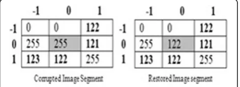
In this example, the pixel to be processed p (x, y) is 255. It is considered as noisy and hence either case 1, 2, or 3 will be performed based on the non-noisy pixel in the current processing window.
Case 1: Initially, the window size is assumed to be 3 × 3. Find the number of non-noisy pixels (k) in the current processing window. Ifkis greater than or equal to three, then find the weights from their positions (−1, 0, 1).
In this example, the number of non-noisy pixels in the current processing window is k= 4. The algorithm requires at least three pixels for interpolation. Hence, interpolate the values using inverse distance weighted interpolation filter. Find the inverse distance of the non-noisy pixels using its pixel position (−1, 0, 1) with respect to the position of the pixel to be proc-essed. The pixel position of 122 in the first row is (1,
−1). The inverse distance is calculated using these
above said positions as calculated in d (1).
dð Þ ¼1 1=
0−1
ð Þ
^
2þ0− −ð Þ1^
2^
0:9
¼0:5359
dð Þ ¼2 1=
0−1
ð Þ
^
2þð0−0Þ^
2^
0:9
¼1
dð Þ ¼3 1= 0− −ð Þ1
^
2þð0−1Þ^
2^
0:9
¼0:5359
dð Þ ¼4 1=
0−0
ð Þ
^
2þð0−1Þ^
2^
0:9
¼1
(ii) Find the sum of the inverse distance.
sum¼Xd ið Þ ¼0:5359þ1þ0:5359þ1¼3:0718
(iii) Divide all the inverse distance by sum which results in the weights of the non-noisy pixels.
v 1ð Þ ¼0:1745;v 2ð Þ ¼0:3255;v 3ð Þ ¼0:1745;v 4ð Þ
¼0:3255
(iv) Interpolate the values by multiplying the weights with the corresponding non-noisy pixels in the current processing window.P(255) refers to the noisy pixel.
Pð255Þ ¼Pv ið Þ g ið Þ
¼0:1745122þ0:3245121þ0:1745
123þ0:3245122¼121:6≈122
The noisy pixel is replaced by 122 as shown in Fig. 2. Case 2: Initially, the window size is assumed to be 3 × 3 as shown in Fig. 3. Find the number of non-noisy pixels (k) in the current processing window.
If k is equal to 2, then increase the window size by 2 to get the window size 5 × 5 and then find the weights from their positions of non-noisy pixels. In this example, the number of non-noisy pixels (k) in
the current processing window is 2. So the window size was increased from 3 × 3 to 5 × 5 as shown in Fig. 4.
The expanded window consists of four numbers of non-noisy pixels. Hence, estimate the processed pixel using inverse distance weighted interpolation filter as shown below. Find the inverse distance of the non-noisy pixels using its pixel position (−2, −1, 0, 1, 2) with respect to the position of the pixel to be proc-essed. The pixel position of 127 in the first row is (−2, −2). The inverse distance is calculated using these above said positions as calculated in d (1).
(i) Find the inverse distance of non-noisy pixel from the center pixel.
dð Þ ¼1 1= 0− −ð Þ2
^
2þ0− −ð Þ2^
2^
0:9
¼0:1539
dð Þ ¼2 1= ð0−1Þ
^
2þ0− −ð Þ1^
2^
0:9
¼0:5359
dð Þ ¼3 1= 0− −ð Þ2
^
2þð0−1Þ^
2^
0:9
¼0:2349
dð Þ ¼4 1=
0−0
ð Þ
^
2þð0−1Þ^
2^
0:9
¼1
(ii) Find the sum of the inverse distance.
sum¼Xd ið Þ ¼0:1539þ0:5359þ0:2349þ1
¼1:9247
(iii) Divide all the inverse distance by sum which results in the weights of the non-noisy pixels.
v 1ð Þ ¼0:08;v 2ð Þ ¼0:2784;v 3ð Þ ¼0:1220;v 4ð Þ
¼0:5196
(iv) Interpolate the values by multiplying the weights with the corresponding non-noisy pixels in the current processing window.P(0) refers to the noisy pixel.
P 0ð Þ ¼Xv ið Þ z ið Þ ¼0:08127þ0:2784126þ0:1220 127þ0:5196129¼127:76¼≈128:
The corrupted pixel is replaced by 128 as shown in Fig. 4.
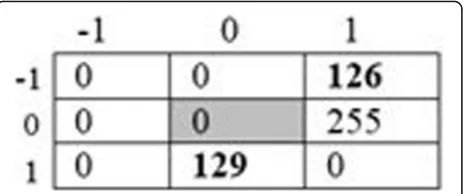
Case 3: Initially, the window size is assumed to be 3 × 3 as shown in Fig. 5. Find the number of non-noisy pixels (k) in the current processing window.
If kis equal to 1, then increase the window size by 4 to get the window size 7 × 7 and then find the weights from their positions of the non-noisy pixels. In this ex-ample, the number of non-noisy pixels in the current processing window isk= 1. So the window size was in-creased from 3 × 3 to 7 × 7 as shown in Fig. 6.
The increased window will now consist of increased non-noisy pixels. Now, the number of non-noisy pixels increased to 7. Hence, interpolate the values using in-verse distance weighted interpolation filter. Find the inverse distance of the non-noisy pixels using its pixel position (−3,−2,−1, 0, 1, 2, 3) with respect to the pos-ition of the pixel to be processed. The pixel pospos-ition of 129 in the second row is (1,−2). The inverse distance is calculated using these above said positions as calculated ind(1).
(i) Find the inverse distance of non-noisy pixel from the center pixel.
Fig. 3Example of corrupted image segment for case 2 of case A
dð Þ ¼1 1=
0−1
ð Þ
^
2þ0− −ð Þ2^
2^
0:9
¼0:2349
dð Þ ¼2 1= ð0−2Þ
^
2þ0− −ð Þ2^
2^
2:9
¼0:1539
dð Þ ¼3 1= ð0−3
^
Þ 2þ0− −ð Þ2^
2^
0:9
¼0:0994
dð Þ ¼4 1=
0−1
ð Þ
^
2þð0−1Þ^
2^
0:9
¼0:5359
dð Þ ¼5 1=
0−2
ð Þ
^
2þð0−1Þ^
2^
0:9
¼0:2349
dð Þ ¼6 1= 0− −ð Þ1
^
2þð0−3Þ^
2^
0:9
¼0:1259
dð Þ ¼7 1=
0−0
ð Þ
^
2þð0−3Þ^
2^
0:9
¼0:1358
(i) Find the sum of the inverse distance.
sum¼0:2349þ0:1539þ0:0994þ0:5359þ0:2349þ0:1259
þ0:1358¼1:5233
(ii) Divide all the inverse distance by sum which results in the weights of the non-noisy pixels.
v 1ð Þ ¼0:1542;v 2ð Þ ¼0:1010;v 3ð Þ ¼0:0653;v 4ð Þ
¼0:3518;v 5ð Þ ¼0:1542;v 6ð Þ ¼0:0826;v 7ð Þ
¼0:0909
(iii) Interpolate the values by multiplying the weights with the corresponding non-noisy pixels in the current processing window.P(0) refers to the noisy pixel.
Pð Þ ¼0 Xv ið Þ g ið Þ
¼0:1542129þ0:1010126þ0:0653126 þ0:3518129þ0:1542126þ0:0826 124þ0:0909121
¼126:8983≈127:
The noisy pixel is replaced by 127 as shown in Fig. 6. Case 4: Initially, the window size is assumed to be 3 × 3 as shown in Fig. 7.
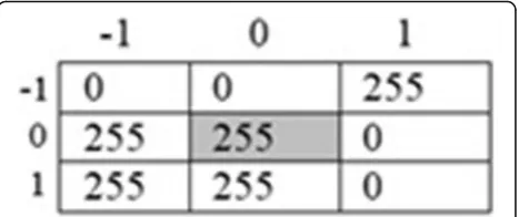
Find the number of non-noisy pixels (k) in the current processing window. If k is equal to 0, then increase the window size by 6 to get the window size 9 × 9 and then find the weights from their positions of non-noisy pixels. In this example, the number of non-noisy pixels in the current processing window is k= 0. So the window size was increased from 3 × 3 to 9 × 9.
The window size is increased to 7, resulting in in-creased number non-noisy pixels to 4. Hence, estimate the new pixel values using inverse distance weighted interpolation filter. Find the inverse distance of the non-noisy pixels using its pixel position (−4,−3,−2,−1, 0, 1, 2, 3, 4) with respect to the position of the pixel to be processed. The pixel position of 129 in the second row is (−3,−4). The inverse distance is calculated using these above said positions as calculated ind(1).
(i) Find the inverse distance of non-noisy pixel from the center pixel.
dð Þ ¼1 1= 0− −ð Þ3
^
2þ0− −ð Þ4^
2^
0:9
¼0:0552
dð Þ ¼2 1= 0− −ð Þ1
^
2þ0− −ð Þ3^
2^
0:9
¼0:1259
dð Þ ¼3 1=
0−2
ð Þ
^
2þ0− −ð Þ1^
2^
0:9
¼0:2349
dð Þ ¼4 1= ð0−4Þ
^
2þð0−1Þ^
2^
0:9
¼0:0076
(ii)Find the sum of the inverse distance.
sum¼Xd ið Þ ¼0:0552þ0:1259þ0:2349þ0:0076
¼0:4236
(iii) Divide all the inverse distance by sum which results in the weights of the non-noisy pixels.
v 1ð Þ ¼0:1303;v 2ð Þ ¼0:2972;v 3ð Þ ¼0:5546;v 4ð Þ
¼0:0180
(iv) Interpolate the values by multiplying the weights with the corresponding non-noisy pixels in the current processing window.P(0) refers to the noisy pixel.
Fig. 6Illustration of case 3 in case A
Pð Þ ¼0 Pv ið Þ g ið Þ
¼0:1303129þ0:2972126þ0:5546121
þ0:0180123
¼123:57≈124
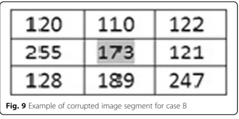
The noisy pixel is replaced by 124 as shown in Fig. 8. Case B: Pixel was not found to be non-noisy, and hence, the pixel is left unaltered.
In this case, the pixel to be processed is 173 which lie between 0 and 255. Hence, the pixel is termed as non-noisy and left unaltered as shown in Fig. 9.
5 Simulation results and discussions
The inverse distance weighted interpolation filter is eval-uated based on different metrics such as peak signal-to-noise ratio (PSNR), image enhancement factor (IEF), and error rate which is given in Eqs. 3, 5, and 6, respectively. The metrics mean squared error (MSE) is given in Eq. 4. The structural similarity index metrics (SSIM) is calcu-lated on various windows of an image. The measure
be-tween two windows x and y of common size MXN is
given in Eq. 7.
PSNR¼10 log10 255 2
MSE
ð3Þ
MSE¼ P
i
P
j
rij−xij
2
MN ð4Þ
IEF¼ P
i
P
j
nij−rij
2
P
i
P
j
xij−rij
2 ð5Þ
Error Rate¼ ½#C
MN100% ð6Þ
Whererrefers to original image,ngives the corrupted image, x denotes restored image, M × N is the size of processed image. C refers to number of restored pixels not equal with original pixels in restored and original image, respectively.
SSIMðx;yÞ ¼ð2μxμyþC1Þð2σxyþC2Þ
μx2þμy2þC2
ð Þ ð7Þ
Where x refers to original image,y refers to restored image, μx is the average of x, μy is the average of y, σx
standard deviation ofx,σyis the standard deviation ofy.
C1 = (K1 L)2 and C2 = (K2 L)2 are two variables to
stabilize the division with weak denominator; L is the dynamic range of the pixel values (for an 8-bit image, it takes from 0 to 255),K1 = 0.01, andK2 = 0.03 by default [28]. The edge preservation performance of the pro-posed algorithm is evaluated using Pratt’s figure of merit (Pratt’s FOM) [29]. The figure of merit of Pratt, which calculates the alikeness between two edge images, is given in Eq. 8.
Pratt’s FOM¼ 1 MAX KI;ð KBÞ
XKB 1
1 1þ∝di2
ð8Þ
where KI and KB are the different points of edges in the restored image and original image, respectively,diis the distance between an edge pixel and the nearest edge pixel of the original and α is a constant and was used α = 1/9, optimal value established by Pratt in [29]. The algorithms used in this paper are derived from the refer-ences cited in the square brackets below. The existing al-gorithms used for the comparison are standard median filter of window size 3 (SMF (3 × 3) [30], adaptive me-dian filter (AMF) (Wmax= 39) [6], center-weighted
me-dian filter (CWF) [7], progressive switched median filter (PSMF) [10], modified decision based median filter (MDBMF) [16], alpha-trimmed mean filter (ATMF) (trimming factor is 4) [30], decision based algorithm (DBA) [13], cascaded filters (CUTMF, CUDBMPF) [15],
Fig. 8Illustration of case 4 in case A
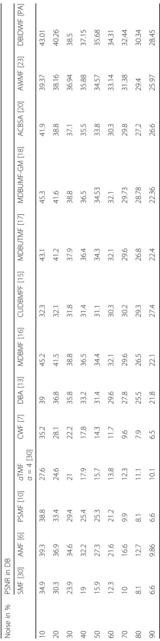
Table 1 Performance of various algorithms at different noise densities for PSNR on Lena image corrupted by SPN Noise in % PSNR in DB SMF [ 30 ]A M F [ 6 ] PSMF [ 10 ] α
TMF α=4[
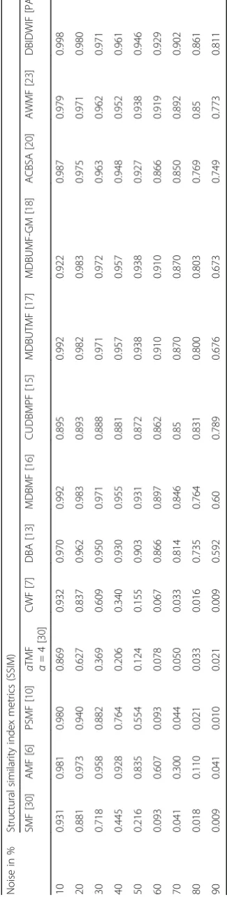
Table 2 Performance of various algorithms at different noise densities for SSIM on Lena image corrupted by SPN Noise in % Structural similarity inde x me trics (SSIM) SMF [ 30 ]A M F [ 6 ] PSMF [ 10 ] α
TMF α=4[
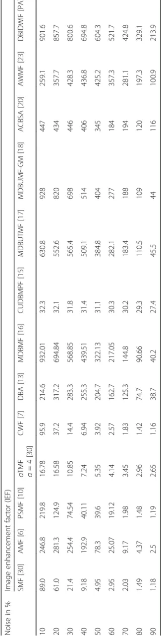
Table 3 Performance of various algorithms at different noise densities for MSE on Lena image corrupted by SPN Noise in % Image enhan cement fact or (IEF) SMF [ 30 ]A M F [ 6 ] PSMF [ 10 ] α
TMF α=4[
modified decision based unsymmetric trimmed median filter (MDBUTMF) [17], improved decision based me-dian filter (IDBA) [14], noise adaptive fuzzy switching median (NAFSM) [31], modified decision based unsym-metrical trimmed median filter with global mean MDBUTMF-GM [18], adaptive cardinal B-spline algo-rithm (ACBSA) [20], and adaptive weighted mean filter (AWMF) (Wmax = 39) [30]. All the algorithms used in
the paper were tested on Kodak natural image database hosted in University of Southern California and Signal and Image Processing Institute website [32]. The images used in the paper are based on the varying information content contained in it. Images such as Lena, camera-man, boat, peppers, and baboon were showcased in the paper as part of the illustration. Exhaustive experiments were conducted, and each algorithm were subjected to different images of the database. All the experiments of the quantitative analysis were done by varying the noise densities in the images from 10 to 90%. All the simula-tion was done in second-generasimula-tion i3-2350 CPU with an operating frequency of 2.30 GHz with a 4GB RAM capability. Tables 1, 2, 3, 4, and 5 give the performance of various algorithms at different noise densities on Lena image corrupted by salt and pepper noise for peak signal-to-noise ratio (PSNR), SSIM, IEF and Pratt’s FOM, respectively. The effectiveness of the algorithm in eliminating noise is decided by PSNR, IEF, and SSIM. The edge preservation capability is checked using Pratt’s FOM. The efficiency of the algorithm in correctly identi-fying noisy pixel from noise free is given by error rate. From Table 1, it is vivid that the algorithm exhibits ex-cellent noise suppression capabilities by offering very good PSNR at high noise densities. Table2 exhibits ex-cellent structural preservation characteristics of the pro-posed algorithm when compared to other standard and
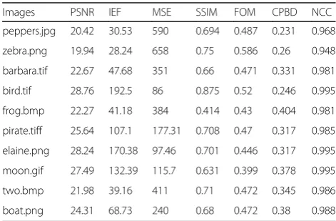
existing algorithms. Table 3 shows a very low value for mean squared error for the proposed algorithm in com-parison with other algorithms. Table 4 illustrates the edge preserving performance (Pratt’s FOM) of the pro-posed algorithm after the removal of salt and pepper noise. The Pratt’s FOM of the proposed algorithm is very high when compared with standard and existing algo-rithms. The proposed algorithm estimates the new pixel values based on the weights generated by inverse dis-tance of the pixels in a small neighborhood with refer-ence to noisy pixel. These weights or uncorrupted pixel of the current processing window has a strong influence on the new interpolated pixel. These uncorrupted neigh-bors preserve the originality of the corrupted pixel. This makes the proposed algorithm to have excellent quanti-tative results. From Tables1,2, and3, we infer that algo-rithms such as SMF, PSMF, trimmed mean filter (TMF), and CWF fail to eliminate noise at high noise densities. Hence, for further analysis, the algorithms were not con-sidered. Table 5 indicates the error rate of various weighted nonlinear filters while removing high density salt and pepper noise. Experiments were conducted to test the efficiency of various weighted algorithms in terms of error rate. It was found that the proposed algo-rithm induces less error when compared to the adaptive cardinal B-spline algorithm and adaptive weighted mean algorithm. The same trend continues even at high noise densities, making the proposed algorithm very good for salt and pepper noise removal. Table6 gives the quanti-tative performance of the proposed algorithm on differ-ent images. Few additional measures were used to illustrate the performance of proposed algorithm such as cumulative probability of blur detection (CPBD) (no ref-erence metrics) and normalized cross-correlation (NCC) (similarity based metrics). The value of the CPBD indi-cates that even without the reference image (original image), the algorithm performs well. The NCC value
Table 5Performance of various weighted algorithms at different noise densities in detecting error rate on Lena image corrupted by SPN
ND in % Error rate in %
AMF [6]
NAFSM [31]
ACBSA [20]
ACWMF [23]
DBIDWIF [PA]
10 20.52 8.55 8.72 10.39 8.29
20 24.53 17.07 17.36 18.35 16.77
30 30.45 25.96 26.19 26.28 25.37
40 37.33 34.47 35.12 34.54 33.9
50 45.29 43.18 43.66 43.08 42.51
60 53.81 52 53.57 52.07 51.3
70 62.77 61.13 62.48 61.31 60.35
80 72.23 70.18 71.47 71.21 69.61
90 82.39 80.16 81.38 82.32 79.65
Table 6Quantitative performance of the proposed algorithm on different images corrupted by 90% salt and pepper noise
Images PSNR IEF MSE SSIM FOM CPBD NCC
peppers.jpg 20.42 30.53 590 0.694 0.487 0.231 0.968
zebra.png 19.94 28.24 658 0.75 0.586 0.26 0.948
barbara.tif 22.67 47.68 351 0.66 0.471 0.331 0.981
bird.tif 28.76 192.5 86 0.875 0.52 0.246 0.995
frog.bmp 22.27 41.18 384 0.414 0.43 0.404 0.981
pirate.tiff 25.64 107.1 177.31 0.708 0.47 0.317 0.985
elaine.png 28.24 170.38 97.46 0.701 0.446 0.317 0.995
moon.gif 27.49 132.39 115.7 0.631 0.399 0.378 0.995
two.bmp 21.98 39.16 411 0.71 0.472 0.345 0.986
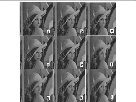
indicates the similarity of the restored image with ori-ginal image even after the removal of high density salt and pepper noise. Figure 10 shows the visual result of the proposed algorithm over the existing and standard algorithms on Lena image corrupted by 90% salt and pepper noise. Figure 11 briefs the qualitative perform-ance of the proposed algorithm over the other algo-rithms on synthetic image corrupted by 90% salt and pepper noise. It was found from Fig. 10 that the pro-posed algorithm exhibits good visual quality when com-pared to other algorithms. Figure11is a synthetic image built using 21 different visual gray levels by a common eye. The information preservation (edges and fine de-tails) of the images is quantified from various edge re-gions (line step and roof edge) of a synthetic image. The edge preservation of the proposed algorithm is explained by considering edges (information of the image) as line edge, ramp edge (semi constant region), step edge (con-stant region), and roof edge, respectively [22]. The pro-posed algorithm attenuates line, step, and roof edge, but
preserves the semi-constant area (ramp edge). On care-ful observation from the synthetic images, it was found that the algorithms such as DBA, IDBA exhibits streak-ing, AMF attenuates edges completely, MDBUTMF also blurs the edges, and spline interpolation filter exhibits edge jittering. NAFSM does not remove salt and pepper noise completely. AWMF also eliminates step edge (first two regions of black and gray). The proposed algorithm showed better detail preserving capability than other al-gorithms because it attenuates the line edges (last two white regions) but preserves ramp edges (varying regions horizontally) even at high noise densities. At high noise densities, existing algorithms exhibits good noise sup-pression characteristics but induce blurring, smearing, streaking, and fading effect as seen in AMF, DBA, and MDBUTMF, respectively. The proposed algorithm gives excellent noise suppression capability without inducing any artifacts (blurring, smearing, streaking, and fading effect). Figure 12 gives the qualitative performance of various weighted algorithms corrupted by 90% salt and
Fig. 13Average PSNR and IEF for various algorithm corrupted by salt and pepper noise on different images
pepper noise on boat, pepper, and baboon image. It was found that proposed algorithm exhibits good noise re-moval capabilities. Existing weighted techniques such as AWMF attenuate edges at high noise densities. The max-imum size of the window used in AMF and AWMF is 39. A larger window size blurs the image. In proposed algo-rithm, the window size is varied depending upon the non-noisy content of the current processing window. Figure13
gives the average PSNR and IEF of different algorithms on different images. Figure 14illustrates the performance of the proposed algorithm on different images such as boat, Lena, and baboon for different images for the quantitative measure MSE and SSIM. Figure 15 gives the frequency spectrum of the different weighted methods on boat
image corrupted by 90% salt and pepper noise. The pro-posed method is compared with the frequency response of ideal low-pass filter. An ideal low-pass filter should have a narrow central lobe. After filtering the restored image, it is subjected to discrete Fourier transform (DFT) and the fre-quency spectrum is plotted. It was found that for the pro-posed algorithm has a narrow central lobe in the spectrum (which is desired for any good filter). From the observation, other adaptive weighted methods such as AMF, NAFSM, and AWMF have a broader central lobe (in comparison to proposed algorithm). This makes the proposed weighted interpolation better than other weighted methods as their frequency response is closer to ideal low-pass filter.
Fig. 15Frequency spectrum of different adaptive weighted methods on Boat image corrupted by 90% salt and pepper noiseaDBIDWIF,b ACBSA,cNAFSM,dAMF, andeAWMF
6 Conclusion
A decision based inverse distance weighted interpolation filter for the elimination of high density salt and pepper noise in images is proposed. The proposed algorithm uses the inverse distance from non-noisy pixels inside the current processing window to estimate the new pixel. This method requires at least three pixels for esti-mation of new pixels, failing which method uses an adaptive window based on the noisy content of the current processing window. The proposed algorithm shows a very good performance due to the usage of in-verse distance of non-noisy pixel in the current process-ing window for estimatprocess-ing new pixels. The interpolation technique is applied to an image only if the processed pixel is noisy. The proposed filter was applied on differ-ent images and found to show very high PSNR, SSIM, and IEF with good computational time supporting with excellent noise removal capability. The information pre-serving capability of the proposed algorithm is justified with an excellent Pratt’s FOM value even at high noise densities. The low error rate indicates the efficiency of the proposed algorithm in restoring the original image. The central lobe in the frequency spectrum of the re-stored image is narrow, thereby making the proposed al-gorithm suitable for noise removal. The proposed algorithm eliminates standard and existing algorithms in terms of excellent noise suppression and good detail preservation without leading to any ambiguity at very high noise densities.
Acknowledgements
The authors would like to thank the Management of Vidya Jyothi Institute of Technology, Aziz nagar, Chilukur Road, Hyderabad-75, Telengana, India for providing us with the infrastructure to complete the research work.
Funding
The research is done by the author himself, and there is no role of funding body involved in the design of the study and collection, analysis, and interpretation of data and in writing the manuscript.
Availability of data and materials
Data will not be shared, reason for not sharing the data and materials is that the work submitted for review is not completed. The research is still ongoing, and those data and materials are still required by the author and coauthors for further investigations.
Authors’contributions
VK is involved in concept, design, acquisition of data, and initial and final analysis. GP is involved in detailed analysis of the code and manuscript drafting (after review). HK is involved in detailed interpretation and manuscript drafting (after revision). VS is involved in code development and initial analysis. All authors read and approved the final manuscript.
Authors’information
Vasanth Kishore Babu received Electronics and Communication from Arulmigu Kalasalingam College of Engineering affiliated to Madurai Kamaraj University with first-class distinction in 2003. He later got M.E degree in Ap-plied Electronics from Sathyabama University in the year 2007 securing uni-versity Fifth rank. He completed his PhD from the same uniuni-versity in the year 2014. He acted as the project leader with the prestigious Sathyabama Nano Satellite for the 25-year-old Sathyabama University. He currently works as a professor of the Department of Electronics and Communication Engineering
at Vidya Jyothi Institute of Technology, Hyderabad, India. His current research interests include non-linear filtering, image enhancement, VLSI signal pro-cessing for image propro-cessing algorithms, and space-qualified systems. He has published more than 50 research papers in reputed journals and conference proceedings.
Ganesan Packyanathan received his BE degree in Electronics and
Communication Engineering from Madurai Kamaraj University, India, in 1998 and ME in Electronics and Control Engineering and PhD degree in Image Processing from Sathyabama University, India, in 2007 and 2015, respectively. Currently, he is a professor of the Department of Electronics and
Communication Engineering at Vidya Jyothi Institute of Technology, Hyderabad, India. His research interests include image processing, soft computing, computer vision, and medical image analysis. He has published more than 50 papers in various journals and refereed conferences. Harikrishna Kamatham obtained his B.Tech in Electronics and
Communication Engineering from Jawaharlal Nehru Technological University Hyderabad and later moved to USA for his Master of Science degree in Electrical and Computer Engineering from Southern Illinois University Carbondale, IL, USA. He has completed his PhD degree in
Telecommunication Engineering from SRM University, Chennai in 2013. His areas of interest include embedded systems, VLSI, and wireless
communications. He is currently working in Vidya Jyothi Institute of Technology as a professor and head of ECE. He has published more than 20 papers in National and International Conferences and journals.
Vishnu Shankar is currently working as an analyst at Verizon Data Services, Chennai India. His research field includes computer vision for robots, non-linear filtering, and mathematics for computer vision. He has won several lau-rels at Maths Olympiad at IIT.
Ethics approval and consent to participate Not applicable.
Consent for publications Not applicable.
Competing interests
The authors declare that they have no competing interests.
Publisher’s Note
Springer Nature remains neutral with regard to jurisdictional claims in published maps and institutional affiliations.
Author details
1Department of E.C.E, Vidya Jyothi Institute of Technology, Aziz Nagar Gate, Chilkur Road, Hyderabad, Telangana 500075, India.2Verizon Data Services, SIDCO Industrial Estate, Guindy, Tamilnadu, India.
Received: 15 May 2015 Accepted: 13 September 2017
References
1. M. Hanumantharaju, M. Ravishankar, D.R. Rameshbabu, S. Ramachandran,
Color Image Enhancement Using Multiscale Retinex with Modified Color Restoration Technique, Second International Conference Proceedings on Emerging Applications of Information Technology (2011), p. 93–97 2. Z. Min, W. Jiechao, L. Zhiwei, L. Yonghua,An adaptive image zooming
method with edge enhancement, 3rd International Conference Proceedings on Advanced Computer Theory and Engineering (2010), p. 608–611 3. W.-S. Tam, C.W. Kok, W.C. Siu, A modified edge directed interpolation for
images. Elec. Imag. J.19(1), 1–20 (2010)
4. W. Bender, C. Rosenberg, Image enhancement using non-uniform sampling. Proc. SPIE-Int. Soc. Opt. Eng.1460, 59–70 (1991)
5. T.S. Huang, G.J. Yang, Fast two dimensional median filtering algorithm. IEEE Trans. Acoust. Speech Signal Process27, 13–18 (1979)
6. H. Hwang, R.A. Haddad, Adaptive median filters: new algorithms and results. IEEE Trans. Image Process4, 499–502 (1995)
7. S.J. KO, Y.H. Lee, Center weighted median filters and their application to image enhancement. IEEE Trans. Circuits Syst.38(9), 984–993 (1991) 8. D.R.K. Brownrigg, The weighted median filter. Commun. ACM27(8),
9. T. Chen, K. Ma, Tri-state median filter for image de-noising. IEEE Trans. Image Process8(12), 1834–1837 (1999)
10. Z. Wang, D. Zhang, Progressive switching median filter for removal of impulse noise from highly corrupted images. IEEE Trans. Circuits Syst. II46, 78–80 (1999) 11. H. Eng, K. Ma, Noise adaptive soft-switching median filter. IEEE Trans. Image
Process10(2), 242–251 (2001)
12. H. Raymond, C.-W.H. Chan, M. Nikolova, Salt and pepper noise removal by median—type noise detectors and detail preserving regularization. IEEE Trans. Image Process14(10), 1479–1485 (2005)
13. K.S. Srinivasan, D. Ebenezer, A new fast and efficient decision-based algorithm for removal of high-density impulse noises. IEEE Signal Process Lett.14(3), 189–192 (2004)
14. M.S. Nair, K. Revathy, R Tatavarti,An Imroved Decision Based Algorithm for Impulse Noise Removal, Proceedings in Congress on Image and Signal Processing (2008), p. 426–431
15. S. Balasubramanian, S. Kalishwaran, R. Muthuraj, D. Ebenezer, V. Jayaraj,An efficient non linear cascade filtering algorithm for removal of high density salt and pepper noise in image and video sequence, Proceedings in International Conference on control, Automation, communication and Energy Conservation (2009), p. 1–6
16. Aiswarya K., Jayaraj V., Ebenezer D.A.New and Efficient Algorithm for the Removal of High Density Salt and Pepper Noise in Images and Videos, Proceedings in International conference on computer modelling and simulation (2010), p. 409–413
17. S. Esakkirajan, T. Veerakumar, A.N. Subramanyam, C.H. Prem Chand, Removal of high density salt and pepper noise through modified decision based
unsymmetrial trimmed median filter. IEEE Signal Process Lett.18(5), 287–290 (2011) 18. T. Veerakumar, S. Esakkirajan, I. Vennila, An approach to minimize very high
density salt and pepper noise through trimmed global mean. Int. J. Compt. Appl.39(12), 29–33 (2012)
19. K. Vasanth, V.J. Senthilkumar, A decision based asymmetricsal trimmed mid point algorithm for the removal of high density salt and pepper noise. App. Theo. Info Tech. J.42(2), 553–563 (2012)
20. P. Syamala Jayasree, P. Raj, P. Kumar, R. Siddavatam, S.P. Ghrera, A fast novel algorithm for salt and pepper image noise cancellation using cardinal B-splines. Int. J. Signal Image Video Process Springer7(6), 1145–1157 (2012) 21. T. Veerakumar, S. Esakkirajan, I. Vennila, Recursive cubic spline interpolation
filter approach for the removal of high density salt-and-pepper noise. Int. J. Signal Image Video Process Springer8(1), 159–168 (2013)
22. K. Vasanth, V.J.S. Kuma, A decision based neighborhood referred unsymmetricsal trimmed variants filter for the removal of high density salt and pepper noise in images and videos. Int. J. Signal Image Video Process Springer9(8), 1833–1841 (2014)
23. P. Zhang, F. Li, A new adaptive weighted mean filter for removing salt-and-pepper noise. IEEE Signal Process Lett.21(10), 1280–1283 (2014) 24. D.J. Brus, J.J. De Gruijter, B.A. Marsman, R. Visschers, A.K. Bregt, A.
Breeuwsma, J. Bouma, The performance of spatial interpolation methods and choropleth maps to estimate properties at points: a soil survey case study. Environmetrics7(1), 1–16 (1996)
25. E. Hosseini, J. Gallichand, J. Caron, Comparison of several interpolators for smoothing hydraulic conductivity data in South West Iran. Trans. Am. Soc. Agric. Eng.36(6), 1687–1693 (1993)
26. E.H. Isaaks, R.M. Srivastava,Applied Geostatistics(Oxford University Press, New York, 1989)
27. R. Webster, M. Oliver,Geostatistics for Environmental Scientists(Wiley, Chichester, 2001)
28. Z. Wang, A.C. Bovik, H.R. Sheikh, E.P. Simoncelli, Image quality assessment: from error measurement to structural similarity. IEEE. Trans. Image Process
13(4), 102–109 (2004)
29. I.A. Abdou, W. Pratt, Quantitative design and evaluation of enhancement/ thresholding edge detectors. Proc. IEEE67(5), 753–766 (1979)
30. J. Astola, P. Kusmanen,Fundamentals of non linear digital filtering(CRC press,Boca Raton, NewYork 1997)
31. K.K.V. Toh, N.A.M. Isa, Noise adaptive fuzzy switching median filter for salt-and-pepper noise reduction. IEEE Signal Process Lett.17(3), 281–284 (2010) 32. SIPI Image Database, USE Signal and Image Processing Institute, http://sipi.