Rate Control Performance under End-User's Perspective: A Test Tool

(1)

doi:10.1155/2010/524613

Research Article

Rate Control Performance under End-User’s Perspective:

A Test Tool

Cristian Koliver,

1

_{Jean-Marie Farines,}

2

_{Barbara Busse,}

3

_{and Hermann De Meer}

3 1_{Center for Computing and Information Technology, University of Caxias do Sul, P.O. Box 1352, Caxias do Sul, Brazil}

2_{Department of Automation and Systems Engineering, Federal University of Santa Catarina, P.O. Box 476, Florianopolis, Brazil} 3_{Department of Mathematics and Computer Science, University of Passau, Innstrae 43, 94032 Passau, Germany}

Correspondence should be addressed to Cristian Koliver,[email protected]

Received 30 April 2009; Revised 9 November 2009; Accepted 19 January 2010

Academic Editor: Benoit Huet

Copyright © 2010 Cristian Koliver et al. This is an open access article distributed under the Creative Commons Attribution License, which permits unrestricted use, distribution, and reproduction in any medium, provided the original work is properly cited.

The Internet has been experiencing a large growth of multimedia traffic of applications performing over an RTP stack implemented on top of UDP/IP. Since UDP does not offer a congestion control mechanism (unlike TCP), studies on the rate control schemes have been increasingly done. Usually, new proposals are evaluated, by simulation, in terms of criteria such as fairness towards competing TCP connections and packet losses. However, results related to other performance aspects—quality achieved, overhead introduced by the control, and actual throughput after stream adaptation—are difficult to obtain by simulation. In order to provide actual results about these criteria, we developed a comprehensive live video delivery tool for testing RTP-based controllers. In this version of the tool, the video is encoded on the fly in the MPEG-2 standard, but we intend to use the H.264/AVC standard as soon as common PC’s provide enough processing power to encode H.264/AVC live video. The tool allows to easily incorporate new control schemes. In this paper, we describe the tool architecture and some implementation details. We also evaluate the performance of the tool itself, in terms of efficacy, accuracy, and efficiency.

1. Introduction and Motivation

Many end-to-end rate control strategies for real-time mul-timedia applications have been proposed in the last years. Most of them are driven to UDP applications running over

the best eﬀort Internet. They are control systems-like, on

which the server adapts its throughput based on feedback messages from the clients. The messages are sent in short intervals. The goals of the rate control strategies include to avoid network congestion and provide TCP-friendliness

[1]. Since the RTP (Real-time Transport Protocol) was

designed by the IETF (Internet Engineering Tasking Force)

for multimedia communication in the Internet and oﬀers

support for collecting information about network load, packet losses and end-to-end delays, the strategies are usually

based upon this protocol (see, e.g., [2,3]).

Pawlikowski shows in [4] the results of a survey of

over 2246 research papers on the network published in the IEEE journals and conferences. The survey revealed that over 51% of all publications on the network adopt

computer simulation to verify their ideas and report network performance results. As mentioned by Ke et al.

in [5], when evaluating video delivered quality, most of

previous studies adopt a video trace file as video stream source in their simulation environment. The advantage is simplicity because researchers do not know much about the concept of video encoding and decoding. But, in the same time, the researchers could not dynamically change the video encoding parameters because of the same reason. In addition, simulations do not provide results related to performance criteria such as the quality oscillation and the overhead introduced by the controller and the actuator. In this paper, we describe a modular live video delivery tool designed for testing RTP-based rate controllers. It allows to easily incorporate new rate control schemes. We also show the results that the tool can provide and evaluate its

performance in terms of eﬃcacy and eﬃciency.

The paper is organized as follows. The architecture

of the tool is presented in Section 2. In Section 3, we

(2)

the performance of our tool in Section 4. InSection 5, we

review some related work. Finally, in Section 6, we discuss

the results and further work to improve the tool.

2. Architecture

Figure 1depicts the architecture of our video delivery tool. In this figure, there is a single client but the server may multicast

the video stream tomclients. At the server-side, the tool is

formed of four separated modules: the MPEG-2 encoder, the packetizer, the controller, and the actuator.

The encoder compresses the raw video stream (from now

designated as test video) on the fly and hasNQoS parameters

ρp (p = 1, 2, 3,. . .,N) to be set. They have influence on

the stream bit rate (by aﬀecting the compression rate) and

quality. A combination of QoS parameters settings is a QoS

level. Thekth QoS levelLkis anN-tuple

Lk=

ρ1k,ρ2k,. . .,ρNk

, (1)

where k = 1, 2,. . .,I (I is the module of the Cartesian

product of the QoS parameters domains). When the encoder

is set asLk, the expectedstream bit rate isrnk(the nominal

rate) and the quality isqnk(the nominal quality). This latter

metric should reflect the stream quality according to the user perspective. In our tool, it is used to rank QoS levels (see

details inSection 3.1).

The packetizer assembles the MPEG-2 video stream provided by the encoder in RTP packets and delivers them over the network. At the client-side, there are two modules: the depacketizer and the MPEG-2 decoder. The depacketizer converts RTP packets into MPEG-2 elementary streams and provides a feedback to the packetizer through receive report (RR) packets. The packetizer computes and provides the

controller with losses (l) and round trip delay (τ). In the

adaptation instantt, the controller computes thetarget rate

rt(t) providing it to the actuator.

The actuator uses the functionQoSto find a QoS levelLk

whosernkmatchesrt(t). The function is

QoS:rt(t)−→Lk,rnk,qnk

, rnk≤rt(t). (2)

The functionQoS is built from a video designated here as

reference video. The reference video should be of the same kind (but not the same video) as the test video. We should

at least have three diﬀerentQoSfunctions: one built from

an action video, a second one built from a talking head

video, and a third one built from a cartoon video (Diﬀerent

kinds of video contents aﬀect the compression rate and,

consequently, the stream bit rate. The perceived quality of

the video is also aﬀected by the video content.). We suggest

these three types of videos to build three diﬀerent QoS

functions based on the video quality test method proposed in ITU-R BS.116-1 Recommendation, the double-blind triple-stimulus with hidden reference. The division according to the video content into action video, talking head video, and cartoon video is due to that an action video usually contains much larger movement than a talking head video. Hence, viewers may easier perceive the jerky motion with the loss of frames in action video. Cartoons videos, in turn, allow

sudden changes in motion, because users generally expect artificial movements in this type of video. Then, the actuator adjusts the encoder parameters

ρ1,ρ2,. . .,ρN (3)

toρ1k,ρ2k,. . .,ρNk. The configuration of the encoder after

adapting is L(t) = Lk. Each adaptation instant t+ 1, the

actuator measures the encoder throughput betweent−1 and

t (the actual rate achieved after adaption instant t−1 or

ra(t−1)) as well asqa(t−1) (the quality actually achieved

after adapting). These values are provided to the actuator to

tuneQoS. Note that it is expected thatra(t−1)≈rt(t−1)≈

rnjandqa(t−1)≈qnj(Lj=L(t−1)).

During the transmission, the tool collects and stores several data that will permit a rate controller performance analysis, such as: output frame rate, losses, bit rate, and quality variation, at the server side, and frame rate, at the client side.

3. Implementation

In this section, we provide the main implementation details of each module, since some of the achieved results are closely related to the tool design aspects. Furthermore, some ideas used here may be useful for other rate controllers implementations.

3.1. The Controller. The controller can be viewed as a black box whose inputs are the round trip delay and the loss rate and the output is the target throughput. It is implemented as

a periodic task whose period isP. PeriodP is the feedback

period defined by the RTP.

A rate controller may compute rt(t) values slightly

diﬀerent fromrt(t−1) values (less than 50 Kbps), generating

thus highly granular target bit rates. Therefore, practical use of rate controller driven to multimedia applications requires a strategy to configure the application in order to achieve a

throughput similar to the target throughputrt(t) computed

by the controller. In our tool, the strategy is implemented by the actuator, described in the next section.

3.1.1. The Actuator. The actuator is responsible for

config-uring the encoder parameters as Lk in time t, such that

rnk is close (but not greater) to the target throughputrt(t)

provided by the controller.

Since the controller can generate values of the target bit

rates diﬀering by some few Kbps, our main concern in the

actuator design was to define a strategy for providing fine

granularity in terms ofrnkandqnkvalues. Common

strate-gies of actuation focusing on a single quality dimension (e.g., strategies based on frame dropping or quantizer adjustment) are unsuitable, since they provide a very discrete set of bit rates values. The application user perceives such limitation as sudden changes of quality; under the network point of view,

the mapping from rt(t) into a QoS levelLk possibly leads

to the bandwidth underutilization. Thus, we opted to useN

dimensional QoS levels composed by the following

(3)

Raw frames

Encoder Actuator

Encoded frames RTP

packetizer Controller

RTP packets

RR packets

RTP packets

RR packets

Server

Clint Network

RTP

depacketizer _Encoded Decoder frames

Raw frames

qa(t−1)

ra(t−1)

L(t)

rt(t)

τ

l

QoS

Figure1: Video delivery tool architecture.

factor or quantizer (qtz), intra-inter matrix combination

(mqt), DC precision (dcp), and matrix of coeﬃcients (mc f)

(see http://www.mpeg.org/MSSG/tm5/index.html for more details about purpose and influence of these parameters on

the compression process). We run several tests using diﬀerent

set of parameters. The above one was chosen by providing a fine quality/rate granularity.

The actuator selects the QoS levelLkfrom a table denoted

byQoST.QoSTis a table whose entries are tuples as

alsk,mtck,mqtk,qtzk,dcpk,mc fk

,rnk,qnk

, (4)

wherealskis the value of parameteralsin thekth table entry,

mtck is the value of parameter mtc, and so on;rnk is the

nominal throughput of the encoded video stream configured

asLk; andqnkis the nominal quality of this stream given by

the average of the signal-to-noise ratio (SNR). Indeed,QoST

represents QoS and it is an extension of the degradation

path strategy [6–8], an ordered list of available QoS levels

and encodings and their resource requirements (particularly, bandwidth). The list is limited by user’s choices and by hardware constraints. The degradation path varies according

to what the users trade oﬀs are.

3.1.2. Construction of QoST. QoST is automatically built

once for a given server prior to the transmission (note that

diﬀerent power processing servers may generate diﬀerent

values ofrnk). TheQoSTconstruction is an iterative process,

where the same short raw clip (the reference video) is compressed again and again setting the encoder parameters,

in each iterationk, asLk. For each iterationk, the variables

rnk andqnk are computed. Then, the tuple given by (4) is

stored as aQoSTentry.QoSTis stored in a file (referenced as

QoST file), to be used for diﬀerent live video transmissions.

When a video transmission is started, the file is loaded in

the multilist.Figure 2shows a same frame of the reference

video, used to buildQoST for our tests, compressed with the

QoS levels Li (Figure 2(a)) and Lj (Figure 2(b)). Note that

whereasrni≈rnj,qniandqnjare very diﬀerent.

TheQoST magnitude may introduce a non-trivial

over-head when seeking a QoS level Lk such that rnk ≈ rt(t).

In order to reduce this delay,QoST is represented internally

like a multilist whose first level nodes represent throughput subranges. Thus, the complexity of seeking is reduced to the number of subranges rather than the number of QoS levels. We defined the actuator granularity as 25 Kbps steps and 10,000 Kbps as the maximum nominal throughput. The granularity is a constant easily changeable. However, we believe that lower values improve granularity but, on the other hand, they degrade accuracy. Therefore, node 0 represents the throughput subrange [0; 25[ Kbps; node

1 represents [25; 50[; node Π represents the throughput

subrange [Π×25; (Π+1)×25[; the 401st node represents the

subrange [10000;∞[. Each first level nodeΠhas associated

a second level list (sublist) whose π nodes contain tuples

alsi,mtci,mqti,qtzi,dcpi,mc fi,qni(i =1, 2,. . .,π). The

valuernπis not stored but it follows the property

rnπ∈[Π×25; (Π+ 1)×25[. (5)

Sublists are sorted in descendant order byqn.Figure 3shows

the multilist structure. Some first level list nodes may contain an empty sublist; most of the sublists contain thousands of

nodes. During transmission,QoST adjusts itself to the video

which is currently transmitted: at the adaptation instant t,

the qualityqnk and the throughputrnkof the current QoS

levelLk = L(t−1) are recomputed (qnk ← qa(t−1) and

rnk ←ra(t−1)). As a result, a head node of a sublist can

(4)

(a) (b)

Figure 2: Same frame of the reference video when the stream QoS levels are: (a) 1, 4, 62, 2, 8, 2, 1047.86, 8.96 and (b)6, 6, 10, 4, 8, 2, 1045.09, 21.80.

When using the tool for delivering a test video, the actuator runs concurrently with the controller and performs only after the end of a GOP because to change some

parameters during a GOP processing may cause side-eﬀects

(e.g., runtime errors due to absence of enough structures to store macroblocks, since the number of structures allocated depends on the GOP pattern and if they are allocated at the beginning of the GOP processing). Therefore, the actuation period varies according to the GOP time processing and it is often much shorter than the control period, that is,

while the controller does not compute rt(t), the actuator

goes on adapting the encoder bit rate to rt(t−1). From

one standpoint, the actuator works unnecessarily. By using a fine-grained period, however, the actuator constantly tailors

the multilist representing the QoST table to the test video

content, improving the tool accuracy.

3.1.3. Actuation Steps. Let Li be the current QoS level at

instantt−1 (i.e.,L(t−1)=Li). In adaptation instantt, the

actuator receives the estimatedrt(t) value from the controller

and performs the following steps:

(1) seeks a nodeπ such that rt(t) ≥ (π+ 1)×25 and

whose sublist head is the QoS levelLjof highestqnj;

(2) sets the encoder asLj (now, Lj is the current QoS

level);

(3) updates the nominal throughput and quality values

ofLi(rni←ra(t−1) andqni←qa(t−1)).

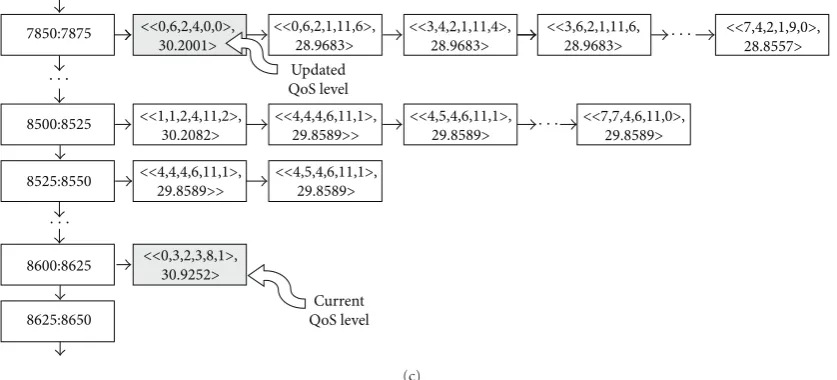
For example, letL(t−1)=Li= 0, 6, 2, 4, 0, 0be the current

QoS level of the stream (seeFigure 3(a)); the current nominal

throughputrn(t−1) is a value between [8525; 8550[ Kbps

and the current nominal qualityqn(t−1)=qniis 30.2154.

Let us suppose that at the adaptation instantt, the controller

computesrt(t)=8612.80. In this case, the actuator:.

(1) seeks, among the first level nodes, that one whose upper limit of subrange is less or equal to 8612.80 (then, the search goes until the subrange [8600; 8625[). The selected QoS level is that one with the highest nominal quality whose node is the

sublist head of the subrange [8600; 8625[ (Lj =

0, 3, 2, 3, 8, 1andqnj=30.9252;Figure 3(b));

(2) sets the encoder asLj(Figure 3(c));

(3) letting 7851.4567 Kbps and 30.2001 dB be, respec-tively, the throughput and the quality measured by

the actuator betweent−1 andt(we mean,ra(t−1)

andqa(t−1)), then it updatesrnito 7851.4567 and

qni to 30.2001. This implies in relocatingLi to the

subrange [7850; 7875[.

3.2. Encoder. The encoder is a modified version of the University of Berkeley’s encoder, which follows the test model 5 (TM5). Since its source code is freely distributed and reasonably well documented, this encoder has been used for educational purposes and as reference for other implementations. We chose an MPEG-1/2 encoder rather than H.264/AVC (more suitable for compression on the fly) due to the simplicity of Berkeley’s encoder code, what makes it easily modifiable. Furthermore, H.264/AVC encoders implemented by software have a very high CPU demand, a critical feature for applications with latency and real time response requirements. The demand is due to the high computational complexity of motion estimation, because of the serial coding nature and high data dependency of coding procedure in both CAVLC and CABAC. When the H.264/AVC encoder use is combined with high resolution video, the only adequate platforms are those with supercom-puting capabilities (e.g., clusters, multiprocessors and special

purpose devices) [9]. However, the other modules of the

tool are reasonably (but not totally) independent from the encoder. Thus, the replacement of the MPEG-1/2 encoder in the tool by another would not be a so hard process (we

describe the main actions required inSection 6).

Originally, the encoder input is a parameter

configura-tion (.par) file with the encoder configuration (resolution,

frame rate, quantization matrices, and so on) and the raw video file name to be compressed; the output is a file containing a MPEG-1/2 stream. We modified the Berkeley’s

encoder so that it supports: (1) variable bit rate (VBR)

(5)

0:25

25:50

1050:1075

<<3,7,60,2,8,4>, 9.0624>

<<0,6,2,1,11,6>, 28.9683>

<<1,1,2,4,11,2>, 30.2082>

<<0,6,2,4,0,0>, 30.2154>

<<0,3,2,3,8,1>, 30.9252>

<<1,1,2,4,8,2>, 29.6843> 1075:1100

7850:7875

8500:8525

8525:8550

8600:8625

8625:8650

8650:8675

10000:∞

<<4,4,4,6,11,1>, 29.8589>> <<4,4,4,6,11,1>,

29.8589>> <<3,4,2,1,11,4>,

28.9683>> <<3,3,62,2,8,0>,

8.9523>

<<3,6,2,1,11,6, 28.9683>

<<6,5,2,0,11,7>, 28.9683>

<<7,4,2,1,9,0>, 28.8557>

<<7,7,4,6,11,0>, 29.8589> <<4,5,4,6,11,1>,

29.8589>

<<4,5,4,6,11,1>, 29.8589>

<<0,4,2,6,11,1>, 33.6111>

<<7,4,,2,3,8,7>, 30.9336> Current QoS level

. . .

(a)

8500:8525

8525:8550

8600:8625

8625:8650

7850:7875 <<0,6,2,1,11,6>,_28.9683>

<<1,1,2,4,11,2>, 30.2082>

<<0,6,2,4,0,0>, 30.2154>

<<0,3,2,3,8,1>, 30.9252>

<<3,4,2,1,11,4>, 28.9683>

<<3,6,2,1,11,6, 28.9683>

<<6,5,2,0,11,7>, 28.9683>

<<7,4,2,1,9,0>, 28.8557>

<<7,7,4,6,11,0>, 29.8589> <<4,4,4,6,11,1>,

29.8589>>

<<4,5,4,6,11,1>, 29.8589>

<<4,4,4,6,11,1>, 29.8589>>

Current QoS level

New current QoS level

<<4,5,4,6,11,1>, 29.8589>

. . .

(b)

(6)

. . . . . .

7850:7875

8500:8525

8525:8550

8600:8625

8625:8650

<<0,6,2,1,11,6>, 28.9683> <<0,6,2,4,0,0>,

30.2001>

<<1,1,2,4,11,2>, 30.2082>

<<4,4,4,6,11,1>, 29.8589>>

<<0,3,2,3,8,1>, 30.9252>

<<3,6,2,1,11,6, 28.9683>

<<7,4,2,1,9,0>, 28.8557>

<<7,7,4,6,11,0>, 29.8589> <<4,4,4,6,11,1>,

29.8589>>

Current QoS level Updated QoS level

<<3,4,2,1,11,4>, 28.9683>

<<4,5,4,6,11,1>, 29.8589>

. . .

(c)

Figure3: Self-adjustment mechanism of the multilist representingQoS.

streams whose target throughput is specified in the par

file. This throughput is achieved adjusting, during the compression process, the quantizer value. Our version gen-erates a VBR stream, since the target throughput generated

by the controller is variable; (2) stream transmission: the

original encoder/decoder are independent programs whose inputs and outputs are files. Our version follows the client-server model. The client-server begins the transmission to a

host (the client) or to a multicast address; (3) command

line configuration: the par file is not used anymore; the encoder configuration can be done by command line. This

modification is needed to automatically generate theQoST

table (afterwards, the configuration is not necessary anymore since the encoder settings change dynamically during video

compression/transmission); (4) mean signal-to-noise ratio

computation:originally, Berkeley encoder computes SNR for

each componentY,U andV of each frame (Y represents

the luminance or luma component of a pixel,UandV the

color diﬀerence components or chroma.). Now, it computes

the mean SNR (SNR) between framesiandi+k(k ∈N∗₎

according to the following equation:

SNR=

i+k

j=iSNRY

j+ SNRU

j+ SNRV

j k+ 1 , (6)

where j is the jth sample (frame), and SNRY(j), SNRU(j)

and SNRV(j) are the SNR values of the frame components

Y,U, and V (SNR(Li) = qni); and (5)mean throughput

computation: the encoder now computes the throughput

between framesjandj+k. This computation is needed for

the creation and the self-adjustment mechanism ofQoST.

3.3. SNR as a Quality Measure. Measuring quality is not always a straightforward process due to the subjective nature of quality. Usually, video quality is evaluated through two

diﬀerent approaches: objective and subjective tests.

The objective tests usually do not take the human perception of the quality into account in their results. It is

well known that the metric used for assessing video quality in our work—SNR—and the peak signal-to-noise ratio (PSNR) are not correlated with human visual system (HVS). A problem of these metrics, based on the mean square error (MSE) computation, is that even though two images may be

diﬀerent, the visibility of this diﬀerence is not considered.

They do not take into consideration any details of the HVS such as its ability to “mask” errors that are not significant to the human comprehension of the image. Cranley et al.

[10] provide an example of this problem. Consider an image

where the pixel values have been altered slightly over the entire image and another image where a small part of the image concentrates all alterations. Both may have the same

MSE value, but they appear to be very diﬀerent to the user.

In addition, SNR does not eﬀectively predict subjective

responses for MPEG video systems. In tests performed by

Nemethova et al. [11], SNR captured only about 21% of the

subjective information that could be captured considering the level of measurement error present in the subjective and objective data.

On the other hand, there is not a consensus about the accuracy of the results provided by traditional video tests methodologies when used for assessing quality for multimedia applications. Watson and Sasse, for example,

argue in [12] that ITU-recommended methods for subjective

quality assessment of speech and video are not suitable, among other reasons, because:

(1) the 5-point quality scales are not viable due to their vocabulary: it is expected the responses to be biased towards the bottom of the scale. The DSCQS permits scoring between the categories (the subject places a mark anywhere on the rating line, which is then translated into a score), but it is still the case that subjects shy away from using the high-end of the scale and will often place ratings on the boundary of the “good” and “excellent” ratings;

(7)

(3) the quality tests typically require the viewer to watch short sequences of approximately 10 seconds in duration, and then rate this material. It is not clear that a 10-second video sequence is long enough to experience the types of degradations common to multimedia applications;

(4) the quality judgments are intended to be made entirely on the basis of the picture quality. It should be queried whether it makes sense to assess video on its own (i.e., without audio), since it would be true to say that the video image in a multimedia application does not have the same importance as in the television system;

(5) results based on the diﬀerence between the degraded

sequence and the reference used for subjective quality

evaluation can diﬀer significantly in some cases

according to the test method, thus also providing limited means for the appropriate quality estimation; and

(6) “one-oﬀ” quality ratings gathered at the end of

an audiovisual session do not capture change of perceptions about the quality that users may have during communication across a packet network with varying conditions.

In our tool, even newer and more suitable testing methodology, driven to quantify multimedia applications quality, are not viable, due to the hundreds of QoS levels

used by theQoSfunction. An alternative to SNR or PSNR

to rank the quality is the video quality metric (VQM) from National Telecommunications and Information

Administra-tion (NTIA,http://www.its.bldrdoc.gov/vqm/), a

standard-ized method of objectively measuring video quality that,

according to the ITU-T [13], closely predicts the subjective

quality ratings that would be obtained from a panel of human viewers. The VQM has the advantage of consisting of

a set of objective metrics, each designed for a diﬀerent target

application.

4. Tool Performance Analysis

Our tool provides data which allow to evaluate the perfor-mance of the rate controller in terms of reduction of losses, smoothness of throughput change, adaptation overhead, and, mainly, video quality achieved. In this section, however, we describe results that permit to evaluate the performance of the tool itself. We used, just as a case-study, a controller following the Enhanced Loss-Delay Algorithm (LDA+),

pro-posed by Sisalem and Wolisz [14]. The LDA+ controller

reg-ulates the server throughput based on end-to-end feedback information about losses, delays and the bandwidth capacity

measured by themclients. This information is sent by the

clients to the server in the RR packets of RTCP protocol. The LDA+ controller uses additive increase and multiplicative decrease factors determined dynamically at the server-side to

computert(t). The factors come from an estimative of the

current network status from the above information (see [14]

for more details aboutrt(t) computation). Note that any

rate controller whose inputs and outputs are those showed inFigure 1could be used to get the data to evaluate the tool performance.

The tool performance is evaluated in terms of its eﬃcacy,

accuracy and eﬃciency.

4.1. Eﬃcacy and Eﬃciency Aspects. A tool for testing rate

controllers should have a mechanism that eﬃcaciously maps

the target bit rate into QoS application parameters, such as the application bit rate matches or is close to the target bit rate. In order to check if our tool reaches this goal, we

measure the error(rt(t),ra(t)), the diﬀerence between the

target bit rate and the bit rate actually achieved.

Another aspect related to the tool eﬃcacy is the achieved

quality. Quality should follow bit rate, that is, the higher bit rate, the higher quality. If quality does not follow bit rate, then the actuator is not selecting the best QoS level for a given target bit rate. In order to evaluate this relationship,

we analyze the behavior ofqa(t) compared tora(t).

In terms of the tool accuracy, we analyze the errors

(rt(t),rn(t)) and(rn(t),ra(t)). Large values of the first

one—the diﬀerence between the target bit rate computed by

the controller and the bit rate selected in the QoST table

by the actuator—indicate that QoST is too coarse. Even if

we have thousands of QoS levels, the set of really useful

QoS levels may be short, since many of them oﬀer the same

quality and/or bit rate. Thus, the granularityde factocan be

known just after generating the multilist representingQoST,

regardless the actuator granularity (25 Kbps; seeSection 3.1).

A coarseQoSTimplies sudden changes of quality, even if the

controller gradually changes the allowed bit rate.

The error (rn(t),ra(t))—the diﬀerence between the

nominal bit rate and the bit rate actually achieved—is due

to the diﬀerences between the reference and test videos.

The scene content influences the compression rates obtained in the temporal and spatial redundancy steps. Therefore, encoded frames of the reference and test videos may present

diﬀerent compression rates even if they are set to the

same QoS level. Large (rn(t),ra(t)) values indicate that

the bit rate values of QoST (rnk) are excessively related

to the reference video. We expect that this error tends to lower during the transmission, due to the self-adjusting

mechanism ofQoST.

Two important aspects related to the tool eﬃciency are

CPU and memory consumption. Since the encoding process has a high CPU and memory usage rate, other tool modules (controller, actuator, and RTP packetizer) should consume a minimum of such resources. Otherwise, it can introduce an overhead in the encoding process increasing the end-to-end delay. In our tool, the most critical data structure in terms of memory requirements is the multilist representing

QoST. Therefore, our focus here is to analyze if it is possible

to reduce its size. For evaluating the overhead introduced by the tool, we compare the response time of the actuator

after receivingrt(t) from the controller, since the most

time-consuming module of the tool—excepting the encoder— is the actuator. (Note that the very high cost process of

(8)

Figure4: Video used in the tests.

the transmission. Furthermore, the same QoST file can be

used for diﬀerent video transmissions).

4.2. Test Environment. In order to evaluate the capabilities of the proposed tool, we conducted a set of transmissions to investigate its performance and to show the data provided by it.

The transmissions were performed using a server host connected to a client host via a router host configured with the RED algorithm to drop packets whenever congestion arises in the network. The physically available bandwidth among the hosts was 100 Mbps, but the server-client link bandwidth was restricted to 6 Mbps, in order to represent a network bottleneck. The reference video used to construct

QoST was a talking heads slow motion clip (the News

clip, see Figure 2). The test video was the Salesman clip

(see Figure 4) (both videos are raw video sequences in the YUV QCIF format publicly available for downloading at http://trace.eas.asu.edu/yuv/) The feedback period is 5 seconds (the RTCP sending interval used by Sisalem and Woliz in the LDA+ tests).

4.3. Results. Figure 5 shows a histogram representing the

QoS levels distribution of QoST for a server with two

hyper-Threading Intel Xeon 2.80 GHz processors. Note that subranges between 1075 and 5000 Kbps concentrate most of the QoS levels. The subranges below 200 Kbps do not have any QoS levels (sublists) associated (and there are some gaps between 200 and 750 Kbps). Therefore, the actuator has to map the target rates below 200 Kbps into the QoS

level Lk such as rnk = 200 Kbps. In a rate controller

of a practical application, this gap could be filled by

buﬀering (e.g., introducing a delay). Indeed, it is possible to

reduce or increase the server throughput through buﬀering,

regardless the QoS level likely CBR applications. However, this approach can lead to an unacceptable end-to-end delay for live video applications.

Figure 6 shows the behavior of rt(t), rn(t) and ra(t).

Note that the behavior of the curvernis close to the behavior

of the curvert. In fact, these variables are strongly correlated:

the correlation coeﬃcient obtained was 0.949 and the P

-value is.0.

The harmonic mean of the absolute values of the errors

(rt(t),rn(t)) is 55.2688 Kbps, a not so large value. As

showed in Figure 7, from time 0 to about 300, the error

2.8 GHz server

×102 100 90 80 70 60 50 40 30 20 10 0

Bit rate (Kbps) 0

20 40 60 80 100 120 140 160 180 200

N

u

mb

er

of

ent

ries

Figure5: QoS levels distribution per throughput subranges (fast server).

×102 14 13 12 11 10 9 8 7 6 5 4 3 2 1 0

Adaptation instantt

0 10 20 30 40 50 60 70

×102

Bi

t

ra

te

(K

b

p

s)

rt(t)

rn(t)

ra(t)

Figure6: Behavior ofrt(t),rn(t) andra(t) during the transmission.

(rt(t),rn(t)) is negative (i.e., rt(t) < rn(t)) because to

t = [0; 300],rt(t)= 0. Thus,rt(t) is mapped intoLj such

as rnj = 200 Kbps. If the initial allowed bit rate was set

at 200 Kbps, then the error int = [0; 300] would be next

to 0. From time t = 300 to the end of the transmission

the error was 0 or positive. This error behavior shows that

rt(t)≥rn(t). The reason is because, in timet, the actuator

selects a QoS levelLksuch thatrnkis close (but never greater)

to the target throughput rt(t) provided by the controller

Section 3.1.1. We used this policy since we believe it is better to underestimate the available bandwidth than taking the risk

of selecting a QoS levelLksuch asrak> rt(t), keeping or even

increasing losses.

The relationship betweenrnandrais also strong, since

the correlation coeﬃcient is 0.911 and theP-value is also.0

(the curvernpractically overlaps the curvera, as showed in

(9)

Harmonic mean: 55.2688

×102 15 14 13 12 11 10 9 8 7 6 5 4 3 2 1 0

Adaptation instantt

−40 −30 −20 −10 0 10 20 30 40

×102

( rt , rn )

Figure7: Error(rt(t),rn(t)).

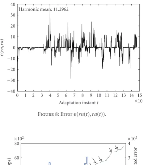
Lk. According toFigure 8, there are some peaks in the error,

probably due to the fact that the reference video background is a ballet scene whereas the test video background is a still

scenario (see Figures2and4, resp.). The diﬀerence between

rnandradecreases during the transmission, due to theQoST

self adjustment mechanism.Figure 9shows the curve rt(t)

and a curve representing the growth of the summed squared

errors(rn(t),ra(t)) (SSErn,ra(t)) during the transmission.

In this figure, some breakpoints in the curve SSErn,ra(t) are

highlighted by arrows. These breakpoints are the beginning

of ranges where SSErn,ra(t) grows slowly. Note that these

ranges correspond to ranges in the curvert(t) whose values

of the target bit rate are equal or similar. The reason is

that the actuator, in a given timet, selects a QoS level Lk

such as rnk ≈ rt(t). The achieved bit rate is ra(t) and

(rn(t),ra(t)) = kt. If in timet+ 1,rt(t) = rt(t+ 1) (or

rt(t)≈rt(t+1)), then the actuator again selectsLk. However,

this turn rnk corresponds to the rate of thernk of the test

video rather than the reference video, thanks to theQoSTself

adjustment mechanism. Therefore,(rn(t+ 1),ra(t+ 1))=

kt+1< kt.

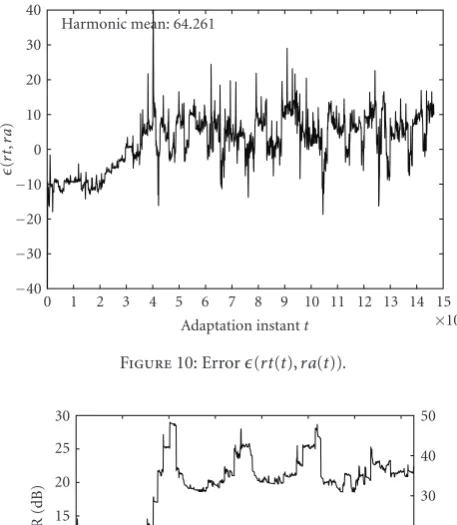
According toFigure 10, the error (rt(t),ra(t)) is often

greater than (rt(t),rn(t)) and (rn(t),ra(t)). This was

expected since

(rt(t),ra(t))=(rt(t),ra(t)) +(rn(t),ra(t)). (7)

In spite of the harmonic mean of|(rt(t),ra(t))|to be more

than twice theQoSTgranularity (64.261 and 25 Kbps, resp.,),

a longer video transmission tends to decrease(rn(t),ra(t))

and, thus, (rt(t),ra(t)). In future work, the value 64.261

may be used as a reference to evaluate other strategies for mapping allowed bit rate into application QoS parameters.

Figure 11also shows the quality (SNR) dynamics during

the transmission. This curve is similar to the the rn(t)

curve of Figure 6. Therefore, quality really follows bit rate,

indicating that the actuator generally selects the QoS level

that better fulfills a given target bit rate.Figure 11also shows

the percentage of packets lost between two RR packets. As expected, there are large quality oscillations, since congestion

×102 15 14 13 12 11 10 9 8 7 6 5 4 3 2 1 0

Adaptation instantt

−40 −30 −20 −10 0 10 20 30 40

×102

( rn , ra )

Figure8: Error(rn(t),ra(t)).

Accumulate error

(rn,ra)

×102 15 14 13 12 11 10 9 8 7 6 5 4 3 2 1 0

Adaptation instantt

0 20 40 60 80

×102

Bi t ra te (K b p s) 0 1 2 3 4

×105

Su m o f ac cum ulat ed er ror

rt(t)

Figure9: Accumulated error(rn(t),ra(t)).

control schemes (such as LDA+) using an Additive-Increase and Multiplicative-Decrease (AIMD) policy produce abrupt bit rate changes. Larger oscillations especially occur in the

presence of losses, whenrt is suddenly decreased. Indeed,

the AIMD policy is not suitable for multimedia applications such as live video and streaming, where a relatively smooth sending rate is of importance. There are rate control mechanisms—for example, the TCP Friendly Rate Control

(TFRC) [15]—more suitable for this kind of applications.

In terms of bit rate adjustment time, Figure 6 shows

that curvert(t) practically overlaps curvera(t),indicating a

trivial control/actuation overhead.

Related to the memory usage,Figure 12shows theQoST

table values rnk ×qnk. Each point in the graph is a QoS

level and they are sorted byrnk. Note that the relationship

between quality and bit rateis notmonotonicly increasing.

This means that inQoSTthere are QoS levelsLiandLjsuch

as

(10)

×102 15 14 13 12 11 10 9 8 7 6 5 4 3 2 1 0

Adaptation instantt

−40

−30

−20

−10 0 10 20 30 40

×102

(

rt

,

ra

)

Figure10: Error(rt(t),ra(t)).

1400 1200 1000 800 600 400 200 0 0 5 10 15 20 25 30

SNR

(dB)

0 10 20 30 40 50

SNR Losses (%)

Figure11: SNR behavior during the video transmission.

that is, there are QoS levels requiring more bandwidth, but

oﬀering an inferior quality than others.Figure 2, for

exam-ple, shows the same single frame of a stream compressed with

two QoS levelsLiandLjwhose entries inQoSTare

1, 4, 62, 2, 8, 2, 1047.86, 8.96,

6, 6, 10, 4, 8, 2, 1045.09, 21.80, (9)

respectively. Whereas rni ≈ rnj, qni and qnj are very

diﬀerent (this is very clear comparing Figure 2(a) and

Figure 2(b)). InFigure 12, a set of dispensable QoS levels is gathered in the rectangle. All of them have a quality equal or lower than the QoS level marked by the arrow but requiring more bandwidth.

Moreover, it is widely accepted the limit of 20 db as a minimum of SNR for a picture to be viewable. Then,

we could also discard QoS levels Lk such as qnk <

20. (The resultant clip is available at http://www.youtube

.com/watch?v=rw7V7U7qDN0 for the reader to draw own conclusions about the end-quality.) Alternatively, we could calculate the minimum transmission bit-rate for a minimum required picture quality based on the Rate Distortion

QoS level Quantizer

10000 8000

6000 4000

2000 0

Bit rate (Kbps) 25

30 35 40 45 50 55

SNR

(dB)

Figure12: Bit rate×quality.

870.6 MHz server

×102 100 90 80 70 60 50 40 30 20 10 0

Bit rate (Kbps) 0

20 40 60 80 100 120 140 160 180 200

N

u

mb

er

of

ent

ries

Figure13: QoS levels distribution per throughput subranges (slow server).

theory [16]. The minimum quality should be preferentially

obtained from subjective tests, despite the controversial

about the accuracy of these tests (see Section 3.3). Levels

bellow the minimum quality can be discarded.

Figure 12 also shows qtz ×rnk. Note that a bit rate

adjustment based only on the quantizer adjustment (a very common approach) cannot smoothly change the bit rate.

Finally, in order to investigate the influence of processing power on the QoS levels distribution among the throughput

subranges, we also generated the QoST table in a slow

server, a Intel Pentium III 870.639 MHz processor.Figure 13

shows a histogram representing the QoS levels distribution

of QoST for this server. QoS levels are predominantly

concentrated between 1500 and 3000 Kbps. The highest throughput is around 5000 Kbps. Note that the QoS levels tend to concentrate on the highest throughput improving the server processing power and vice-versa. Hence, the throughput subrange where a QoS level is placed depends on

(11)

To summarize, the above results indicate that: (1)QoST

provides a large and continuous range of possible through-puts. This is a necessary condition for testing the quality

provided by a rate controller; (2) initial valuesrnk(nominal

rate) and qnk (nominal quality) of the QoS level Lk in

QoST, obtained from the reference video, are a reasonable

approximation of the valuesra(t) and qa(t), the actual bit

rate and quality achieved for the test video when the encoder

is set toLk; (3) the minimum and maximum bit rate [m,M]

bounded by the tool depend on the server processing power. A powerful video server increases both values; (4) quality oscillation occurs due to the rate controller approach used to compute the allowed (target) bit rate. The test tool only tries to reach this target bit rate. If the target bit rate oscillates or/and changes suddenly, then the quality will also oscillate or/and change suddenly; and (5) thousands of QoS levels may be discarded, reducing the tool memory needs.

5. Related Work

Cranley et al. [10] have proposed an optimal way in which

multimedia transmissions should be adapted in response to network conditions to maximize the user-perceived quality. Similar to our work, their approach assumes that within the

set of diﬀerent ways to achieve a target bit rate, there exists an

encoding maximizing the user-perceived quality. Extensive subjective tests suggests that an Optimal Adaptation Tra-jectory (OAT) in the space of possible encoding does exist and that it is related to the content type. In their paper, the authors explore the possibility of applying objective metrics to discover the OAT and compare it to those found through extensive subjective tests.

Diﬀerently from the work of Cranley et al., our work

is not supposed to be a model or architecture for QoS adaptation, but simply a tool for testing and comparing rate controllers. Therefore, it is a support for the research in this area. However, the OAT function could be used in our tool as

a degradation path rather than theQoSfunction.

Yan et al. presents in [17] a media- and TCP-friendly

rate-based congestion control algorithm (MTFRCC) for scalable video streaming on the Internet. To each transmission at

rate rs ∈ [ms,Ms] of a sender s is associated a utility

functionUs(rs). They assume thatUsis twice continuously

diﬀerentiable in [ms,Ms]. The objective of the algorithm

is to choose source rates rs such that the overall utility

is maximized, that is, to optimize the video quality of all streams. It should be noted that the utility function varies according to video coding scheme used. To tailor the utility function to application quality, Yan et al. use the rate-distortion function such as

Us(rs)= −Ds(rs), (10)

where Ds(rs) is the rate-distortion function for finer grain

scalable (FGS) video derived from a mixture-Laplacian

statistical model of FGS video streams proposed in [18] and

given by:

Ds(rs)=2ρ1·rs+ρ2

√

rs+ρ3, ₍₁₁₎

where ρ1, ρ2, and ρ3 are parameters to be empirically

evaluated. They stand for the streaming rate and for the

distortion of a single frame. The values ofρ1,ρ2, andρ3vary

depending on the source video stream. With the availablers−

Dinformation, the values ofρ1,ρ2, andρ3can be computed

during the encoding process, for real-time operation. The values are computed once for each video sequence and it is assumed that they remain constant throughout the entire

streaming process. The rate-distortion function in (11) is

strictly decreasing and convex whereas the utility function in

(10) is strictly increasing and concave. In practice, the raters

has to be, in the congestion avoidance phase, not smaller than

the bit rate of the base layerms; otherwise the application

quality will be significantly harmed and packet delivery will be unacceptably delayed.

TheQoSfunction is similar to theUsfunction, in terms

of purpose and construction. However, in practice, the cost

of determination of theQoSto each QoS levelLkis very high

depending on the encoder parameters compoundingLk; we

again highlight that this process is executed once and the

QoScan be used for diﬀerent video transmissions. On the

other hand,QoSis not bounded to three parameters and can

be more continuous thanUs. Moreover,QoSis tailored to

the video during the transmission, that is, the quality and bit rate associated to the QoS levels do not remain constant throughout the entire video delivery process.

Ke et al. present in [5], a simulation tool integrating

the EvalVid tool-set [19] and NS-2. EvalVid is a

tool-set for evaluating video quality transmitted over a real or simulated communication network. The EvalVid’s purpose is to assist researchers in evaluating their network mechanisms or designed protocols in terms of user-perceived video quality over a real or simulated network. To improve the simulation model, Ke et al. enhanced some interfaces into EvalVid. With the enhancement, the tool-set enables not only network-related researchers to evaluate real video streams on their proposed network designs or protocols, but also video-related researchers to evaluate video quality of their designed video coding mechanisms using a more realistic network. On the one hand, the work is not bounded by testing rate controllers and permits tests without a real environment and controller implementation. On the other hand, the tool set uses encoded video trace files generated from YUV files. This aspect became hard to test controllers based on setting the encoder parameters in real-time.

Lotfallah et al. propose in [20] a framework for advanced

video traces which enables the evaluation of video transmis-sion over lossy packet networks, without requiring the actual videos. The two main components of this framework are (1) advanced video traces which combine the conventional video traces with a parsimonious set of visual content descriptors, and (2) quality prediction schemes that based on the visual content descriptors provide an accurate prediction of the quality of the reconstructed video after lossy network transport. The video traces represent a small number of

encodings (versions) with diﬀerent encoding bit rates for

(12)

correlate with the reconstructed quality). The number of provided QoS levels is bounded by the number of versions, whereas in our work this number is given by the number and the nature of the QoS parameters used.

6. Conclusions and Future Work

In this paper, we described a live video delivery tool that can be used to test RTP-based rate controllers providing complementary results to those ones achieved by simulation. Particularly, it is useful to provide results related to actual achieved quality, overhead introduced by the control, and actual throughput. The tool may aid rate controller designers to test their strategies regarding performance aspects hard to evaluate by simulation (e.g., control overhead, frame rate at the clients, quality achieved, quality oscillation, etc.). Since it is highly modular, the tool can use any controller structured as a black box whose inputs are round trip delay and loss rate and the output is the target throughput.

Our results indicate that (1) the actuator often finds a

nominal throughput close tothe target throughput; (2) the

self adjustment mechanism of QoST satisfactorily corrects

the throughput and quality nominal values of the QoS levels used for rate adapting during the video transmission (note that these values are strongly related to the reference video in the beginning of the transmission); and (3) the encoding/control overhead is not critical in the end-to-end delay when the server answers a single video request.

Even though our tool has been designed and imple-mented to be a tool for RTP-based controller test support, its actuation strategy can be exploited as part of a rate control mechanism of live video delivery tools. Note that it was not our intent to build a fully functional live video application since there are many libraries supporting the development of such applications and even fully functional open source applications. However, to provide support for

diﬀerent encoders, many of them have a large and complex

source code. In addition, some of them generate only CBR streams. Therefore, our tool can be used to test and compare

diﬀerent control approaches prior to the construction of a

live video delivery application with rate control.

Some limitations of the current version of our tool include: use of pre-stored raw video rather than real-time

captured video, absence of client-side buﬀering for

smooth-ing jitter, and MPEG-2 encodsmooth-ing rather than H.264/AVC, which delivers similar quality at lower data rates. However, a future work includes to replace the MPEG-2 encoder by the H.264/AVC Scalable Video Coding (SVC) to define QoS levels in terms of the multi-dimensional scalability provided

by this encoder [21] (previous work on rate control for

H.264/AVC/SVC streams was primarily based on changing resolution layers by using the FGS feature. However, FGS— include in a draft document—has been removed according

to [22].). The use of a VBR H.264/AVC/SVC encoder

performing transmission over an RTP stack rather than the current MPEG-2 would request minor modifications. More precisely, it would be necessary: (1) to identify in the source code the variables used for the encoder settings and

select those ones to compound QoS levels; (2) to allocate them as shared memory assuring mutual exclusion (since the actuator runs concurrently with the encoder); and (3) to identify the relationship of these variables with others and the encoder data structures, especially for variables related to the temporal compression (this is the hardest part!).

A currently practical diﬃculty in using H.264/AVC is the

time demanded by this encoder to compress a video in real-time, when the server is a common PC. We performed some tests on a two processors Intel Pentium CPU 2.80 GHz machine using the JM version 15.0 H.264/AVC encoder

implementation (http://iphome.hhi.de/suehring/tml/). The

frame rate of encoding a raw video (QCIF format, 30 fps, and baseline profile), for example, was less than 1 fps. Neverthe-less, we believe presently common PC’s will provide enough processing power to encode live video in the H.264/AVC standard by software.

Another future work is to test and compare the perfor-mance of more recent TCP-friendly rate control mechanisms

using our tool, such as TFRC [15].

Currently, we are designing a new version of the tool based on the Datagram Congestion Control Protocol (DCCP) rather than RTP over UDP. By using this new version, we will be able to verify the actual video quality

provided by diﬀerent congestion control mechanisms, such

as CCID 2 (Congestion Control ID 2), CCID 3, and CCID 4, when used to transport both streaming applications data as live video data applications.

The resultant video received by the client in the

tests can be viewed at http://www.youtube.com/watch?v=

rw7V7U7qDN0. By watching this video, the reader can draw own conclusions about the quality variation.

References

[1] J.-Y. L. Boudec, “Rate Adaptation, Congestion Control and Fairness: a Tutorial,” 2008.

[2] C. Koliver, K. Nahrstedt, J.-M. Farines, J. D. S. Fraga, and S. A. Sandri, “Specification, mapping and control for QoS adaptation,”Real-Time Systems, vol. 23, no. 1-2, pp. 143–174, 2002.

[3] S. Lee and K. Chung, “TCP-friendly rate control scheme based on RTP,” inProceedings of the International Conference on Information Networking (ICOIN ’06), I. Chong and K. Kawahara, Eds., vol. 3961 ofLecture Notes in Computer Science, pp. 660–669, Springer, Sendai, Japan, 2006.

[4] K. Pawlikowski, “Do not trust all simulation studies of telecommunication networks,” inProceedings of the Interna-tional Conference on Information Networking (ICOIN ’03), vol. 2662, pp. 3–12, Jeju Island, Korea, 2003.

[5] C.-H. Ke, C.-H. Lin, C.-K. Shieh, and W.-S. Hwang, “A novel realistic simulation tool for video transmission over wireless network,” inProceedings of the IEEE International Conference on Sensor Networks, Ubiquitous, and Trustworthy Computing, pp. 275–281, Los Alamitos, Calif, USA, June 2006.

(13)

[7] M. Fry, A. Seneviratne, and V. Witana, “Delivering QoS controlled continuous media on the World Wide,” in Proceed-ings of 4th IFIP International Workshop on Quality of Service (IWQoS ’96), Paris, France, 1996.

[8] G. Ghinea and J. P. Thomas, “Improving perceptual multi-media quality with an adaptable communication protocol,” Journal of Computing and Information Technology, vol. 13, no. 2, pp. 149–161, 2005.

[9] A. Rodriguez, A. Gonzalez, and M. P. Malumbres, “Hier-archical parallelization of an H.264/AVC video encoder,” in Proceedings of the IEEE International Symposium on Parallel Computing in Electrical Engineering (PARELEC ’06), pp. 363– 368, IEEE Computer Society, Los Alamitos, Calif, USA, 2006. [10] N. Cranley, P. Perry, and L. Murphy, “User perception

of adapting video quality,” International Journal of Human Computer Studies, vol. 64, no. 8, pp. 637–647, 2006.

[11] O. Nemethova, M. Ries, E. Siﬀel, and M. Rupp, “Quality assessment for H.264 coded low-rate and low-resolution video sequences,” in Proceedings of the 3rd IASTED International Conference on Communications, Internet, and Information Technology (CIIT ’04), pp. 136–140, St. Thomas, Va, USA, November 2004.

[12] A. Watson and M. A. Sasse, “Measuring perceived quality of speech and video in multimedia conferencing applications,” in Proceedings of the 6th ACM International Conference on Multimedia, pp. 55–60, Bristol, UK, September 1998. [13] ITU-T Recommendation J.149, “Method for specifying

accu-racy and crosscalibration of video quality metrics (VQM),” 2004.

[14] D. Sisalem and A. Wolisz, “LDA+: a TCP-friendly adaptation scheme for multimedia communication,” in Proceedings of the IEEE International Conference on Multi-Media and Expo (ICME ’00), pp. 1619–1622, IEEE Press, New York, NY, USA, July-August 2000.

[15] S. Floyd, M. Handley, J. Padhye, and J. Widmer, “TCP Friendly Rate Control (TFRC): Protocol Specification,” RFC 5348 (Proposed Standard), September 2008.

[16] L. D. Davisson, “Rate-distortion theory and application,” Proceedings of the IEEE, vol. 60, no. 7, pp. 800–808, 1972. [17] J. Yan, K. Katrinis, M. May, and B. Plattner, “Media- and

TCP-friendly congestion control for scalable video streams,”IEEE Transactions on Multimedia, vol. 8, no. 2, pp. 196–206, 2006. [18] M. Dai, D. Loguinov, and H. Radha, “Rate-distortion

model-ing of scalable video coders,” inProceedings of the International Conference on Image Processing (ICIP ’04), vol. 5, pp. 1093– 1096, Society Press, October 2004.

[19] J. Klaue, B. Rathke, and A. Wolisz, “EvalVid—a framework for video transmission and quality evaluation,” inProceedings of the 13th International Conference on Modelling Techniques and Tools for Computer Performance Evaluation, pp. 255–272, Urbana, Ill, USA, 2003.

[20] O. A. Lotfallah, M. Reisslein, and S. Panchanathan, “A framework for advanced video traces: evaluating visual quality for video transmission over lossy networks,”EURASIP Journal on Applied Signal Processing, vol. 2006, Article ID 42083, 21 pages, 2006.

[21] P. Ni, A. Eichhorn, C. Griwodz, and P. Halvorsen, “Fine-grained scalable streaming from coarse-“Fine-grained videos,” in Proceedings of the 18th International Workshop on Network and Operating System Support for Digital Audio and Video (NOSSDAV ’09), pp. 103–108, Williamsburg, Va, USA, June 2009.