On Various Approaches for Bi-level Optimization Problems

http://www.sciencepublishinggroup.com/j/ijmfs doi: 10.11648/j.ijmfs.20190503.11

ISSN: 2575-4939 (Print); ISSN: 2575-4947 (Online)

On Various Approaches for Bi-level Optimization Problems

Mohamed Aly El Sayed

1, *

, Farahat Abdo Allah Farahat

2

1

Department of Basic Engineering Sciences, Benha University, ElQalyoubia, Egypt

2

Higher Technological Institute, Tenth of Ramadan City, Cairo, Egupt

Email address:

*

Corresponding author

To cite this article:

Mohamed Aly El Sayed, Farahat Abdo Allah Farahat. On Various Approaches for Bi-level Optimization Problems. International Journal of Management and Fuzzy Systems. Vol. 5, No. 3, 2019, pp. 47-63. doi: 10.11648/j.ijmfs.20190503.11

Received: September 23, 2019; Accepted: October 18, 2019; Published: October 25, 2019

Abstract:

In this paper we review some different basic approaches for solving bi-level optimization problems (BLOP). Firstly, the formulation and some basic concepts of such BLOP are presented. Secondly, some conventional approaches for solving the BLOP such as; vertex enumeration method, branch and bound algorithm, Karush Kuhn-Tucker (KKT) transformation are exhibited. The vertex enumeration based approaches which use the important characteristic that at least one global optimal solution is attained at an extreme point of the constraints set. The KKT approaches in which a BLOP is transformed into a single level problem that solves the upper level decision maker (ULDM) problem while including the lower level decision maker (LLDM) optimality conditions as extra constraints. Fuzzy programming approach mainly based on the fuzzy set theory. Finally, formulation of the bi-level multi-objective decision making (BL-MODM) problem and recently developed approaches, such as; fuzzy goal programming (FGP) and technique for order preference by similarity to ideal solution (TOPSIS) approach, for solving such problem are presented. Numerical illustrations are presented for each technique to ensure the applicability and efficiency.

Keywords:

Bi-level Programming, Multi-objective Programming, KKT Transformation, FGP, TOPSIS

1. Introduction

Many planning problems require the synthesis of decisions of several interacting individuals or agencies. Often these groups are arranged within a hierarchical administrative structure, each with independent and perhaps conflicting objectives. Multi-level decision making has always been regarded as an important aspect of the planning process [1-5]. Frequently, the impacts of directives from supervisors and reactions from subordinates have been viewed as externalities, beyond the control of planner. However, there have been attempts to model the ability of one planner to indirectly influence the decisions of others to his benefits. The BLOP, which we are interested in our work, are merely a special case of the multi-level decision making problems [6-10]. An important feature of hierarchy structures is that a planner at one level of the hierarchy may have his objective function and decision space determined, in a part, by the other level. In addition, each planner’s control instruments may allow him to influence polices at the other levels and

thereby improves his own objective function. These instruments may include the allocation and use of resources at lower levels, and benefits conferred up on other level.

Literature Review

From the historical point of view, BLOP is closely related to the economic problem of Stackelberg in 1952, in the field of game theory. The original formulation for BLOP appeared in 1973, in a paper authored by J. Bracken and McGill in 1973, it was developed by W. Candler and R. Norton in 1977 who first used the designation "bi-level" programming. However, it was not until the early nineteen eights that these problems started to receive the attention they deserved [11].

upper-level and the lower-level) in a hierarchy. The decision maker (DM) at the upper-level (the leader) firstly optimizes his/her objective function independently. After the leader chooses the decision, the DM at the lower-level (the follower) makes his/her decision. The leader knows the objective and constraint functions of the followers, who may or may not know the objective and (or) constraint functions of the leader. However, the leader’s decision is influenced by the reaction of the follower. Since many practical problems, such as engineering design, management, economic policy and traffic problems can be formulated as hierarchical problems, it is important to solve them effectively. Therefore, many researchers have done intensive research on the theories, methods and applications of the BLOP [1, 3].

The methods for solving the BLOP have received more extensive attention than theories and application separately. The various traditional algorithms to solve the BLOP can be roughly classified into the following categories: Extreme-point approaches for the linear case, Branch and bound algorithm, Parametric Complementary pivoting (PCP), Descent methods, Penalty function methods, Trust-region methods and so on. However, the BLOP is a non-convex problem, and it is extremely difficult to solve it. During the past two decades of last century, several approaches for solving BLOPs have been deeply studied by Candler [12], Bialas and Karwan [14, 15]. Bialas and Karwan are the pioneers for BLOPs who presented vertex enumeration method, called best solution. These were solved by simplex method. To solve the non-linear problem that arises due to the KKT conditions, Bialas and Karwan [15] proposed a parametric complementary pivot (PCP) algorithm which interactively solves a slight perturbation of the system. Ben-Ayed et al. [16] showed that the PCP may not converge to optimality. Among the many approaches for solving the BLOPs, the branch and bound algorithm appears to be one of the more effective approaches among the traditional optimization techniques. In 1981 Fortuny-Amat and McCarl [13] suggested the use of two equality constraints with zero-one variables to replace the non-linear complementary term. In 1982 Bard and Falk [17] proposed the branch and bound algorithm which based on a series of transformation through the complementary slackness condition. Moreover in 1990 Bard and Moore [17] used this concept to improve their earlier branch and bound algorithm.

Due to complexity of the BLOPs, there are no efficient traditional techniques for obtaining the solutions of a reasonable size problem and most of the classical approaches developed so far do not consistently perform well. Moreover, decision deadlock arises in some situations due to rejecting the solution by the follower for not giving a decision power to him/her to reach a minimal level of satisfaction in the decision making situation. To overcome the shortcomings of the classical approaches, Fuzzy Programming (FP) approach to BLOPs, by using the concept of tolerance membership function, was introduced by Lai [18] in 1996. Hence, Shih et al. [19] extended Lai's concept by using non-compensatory max-min aggregation operator for solving multi-level optimization problem (MLOP). Shih and Lee [20] further

extended Lai's concept by introducing the compensatory fuzzy operator for solving MLOP. Sakawa et al. [21] developed interactive FP for solving two-level linear fractional programming problems with fuzzy parameters in 2000. Also, Sakawa et al. [22] proposed Interactive FP for decentralized two-level linear programming problems in 2002.

In 1997 Shi and Xia [23] studied the bi-level Multi-Objective Decision Making (BL-MODM) problem and an interactive algorithm to solve such problem. Abo-Sinna [24] discussed non-linear multi-objective BLOP in fuzzy environment in 2001. Osman et al. [25] in 2004 studied MLOP under fuzziness. In 2006 Abo-Sinna and Baky [26] presented balance space approach for non-linear BL-MODM problem. Zhang et al. [27] presented an algorithm for solving decentralized BL-MODM problem with fuzzy demands by using -cut method. Gao et al [11] studied fuzzy linear BLOP based on -cut and goal programming.

FGP approach to BLOP has been recently studied by Moitra and Pal [28]. In 2003, Pal et al. [29] presented a GP procedure for fuzzy multi-objective linear fractional programming problem. Pramanik and Roy [30] proposed a solution methodology based on FGP for solving MLOPs. In 2009, A. Baky [31] studied FGP algorithm for solving decentralized BL-MODM problems. Also, Baky extended FGP approach to solve ML-MODM [32]. In addition to that Baky et al. presented a FGP procedure for solving fuzzy BLOP [33]. Recently the TOPSIS approach has been extended by Baky and Abo-Sinna to solve the BL-MODM problem [34]. MLOP was as of late concentrated by Chen and Chen [35]. Youness et al. exhibited Fuzzy integer BL-MODM in [36]. A modified TOPSIS method presented by Baky & Elsayed for BLOP with vague numbers [37]. Ranarahu et al. presented method for solving a multi-objective BLOP [9]. Lachhwani in [38] tackled a solution for MLOP based on FGP approach. Ren developed in [39] a method to deal with the fully fuzzy BLOP by applying interval programming notions. An interactive approach for fractional MLOP under fuzziness displayed by Osman et al. [3]. Parametric notions of fractional fuzzy MLOP has been introduced by Osman et al. [2].

The paper is organized as follows: Following introduction, Sect. 2 present some notions and formulation of BLOP. In the next section conventional approaches for solving BLOP. Sect. 4 incorporates BL-MODM problem moreover FGP and TOPSIS for tackling such problem. Finally, some conclusions are incorporated in Sect. 5.

2. Notions and Formulation of Bi-Level

Optimization Problem

A bi-level programming problem can be viewed as a static version of the non-cooperative, two planner game introduced by Von Stackelberg in the context of unbalanced economic markets [11, 17, 18]. The problem we want to consider have the following common chrematistics [15, 17, 40-42]:

a hierarchical structure.

2.Each subordinate level executes its policies after, and views of, the decisions of superior levels.

3.Each unit maximizes net benefits independently of other units, but may be affected by the actions and reactions of those units.

4.The external effect on a DM’s problem can be reflected in both his objective function and his set of feasible decisions.

2.1. Problem Formulation and Definitions

Assume that there are two-levels in a hierarchy structure with Upper-Level Decision Maker (ULDM) and Lower-Level Decision Maker (LLDM). Let a vector of decision variable = , ∈ be partitioned amongst the two planners. The ULDM has control over the vector ∈ ⊂

and the LLDM has control over the vector ∈ ⊂ , where = + . When the policies are finally

executed, level one will first specify , and level two will then specify , with the full knowledge of level one’s decisions. Let ⊂ denote the feasible choices of , . We will assume that is closed and bounded. So the BLOP may be formulated as follows [12, 13, 15, 16, 41]:

[1 ]

!" #

$ % , = & = & + &

'ℎ ) *

[2 , ]

!"#

$ % , = & = & + &

-./ & *

∈ = 0 = , ∈ |2 + 2 ≤ ., , ≥ 0, . ∈ 6_{7 ≠ 9 (1)}

where 2 and 2 are ! × -and ! × dimensional matrices, respectively, & and & are -dimensional vectors, & and & are -dimensional vectors, and is the bi-level convex constraints feasible choice set.

Because of various applications in different fields, different names have been used in literature for the leader. Some of them are upper, outer, level one, or policy. Similarly lower, inner, level two, or behavioral are used instead of follower.

For any fixed choice of , the lower-level will chose a

value of that optimizes its objective function. Hence, for each feasible value of , the lower-level will react with a corresponding value of . This results in a functional relationship between the decisions of the upper-level and the reactions of the lower-level, say = ; . Based on these we have the following definitions [11, 16, 41]:

Definition 1:

The constraint set of the BLOP:

= 0 = , ∈ |2 + 2 ≤ ., , ≥ 0, . ∈ 6_{7 ≠ 9,}

The feasible set for the lower-level for each :

= 0 ∈ , > 0|2 ≤ . − 2 7

The projection of onto the upper-level decision space:

= 0 ∈ |∃ ∈ , 2 + 2 ≤ . 7

The lower-level rational reaction set for ∈ :

;? = 0 ∈ | * : !" [% , '" ℎ ∈ ]7

The inducible region:

A = B , C ∈ , ∈ ;? D

The rational reaction set ;_? defines the response while the inducible region A represents the set over which the ULDM may optimize his objective if he/she has the control over all the variables.

Definition 2: A point , is called feasible solution of

the BLOP if , ∈ ;_? , ∈ .

Definition 3: A point ∗, ∗ is an optimal solution of the BLOP if and only if [11, 16]:

∗_, ∗ _{is a feasible solution of the BLOP,}

For all feasible points , , % ∗, ∗ ≤ % , , For all feasible points ∗, , if & = & ∗ then

& ∗_{= & .}

The third condition states that if the LLDM is in different between ∗ and when is fixed to ∗, then the ULDM must also be in different between ∗, ∗ and ∗, .

2.2. Effects of Multiple Optima

For any BLOP, care must be taken when the solution to the lower-level problem is not unique for fixed . Although not affecting the value of the lower-level objective function, % , these solutions can have a greatly varying impact on the objective at the upper-level. To overcome the problem Bialas and Karwan [17] in 1978, suggested replacing the original lower-level problem by %∗ = % + F% where the value of F > 0 is suitably small, this method perturbs the lower-level problem. This would require that the ULDM share a small portion of its earning to encourage the LLDM to choose a desirable solution to the upper-level objective. In general, to check the effect of multiple optima, we can solve the BLLP problems: once with the lower level objective function equal to % + F% , and a second time with that function equal to % − F% . And optimal solution is obtained if it is optimal in both cases [15, 17].

2.3. Non-Convexity of The BLOP

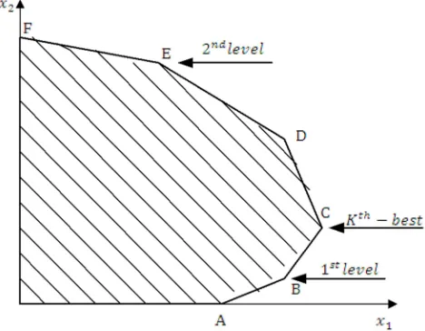
than familiar mathematical programming. For example, consider the BLOP with = , ∈ , ∈ , ∈ . Although its overall feasible region, G , is a convex polyhedron and all objectives are linear, the actual problem is non-convex. In Figure 1, for any fixed choice of , level two will choose the value of which minimizes & &

& . This results in the rational reaction set, G , which is the bold region in Figure 1. The obvious choice of for level one is that which yields the minimum value of & with respect to the bold region. This requires the minimization of a linear objective function over a non-convex set. We conclude that the most significant characteristic of the BLOP is that the feasible region of the ULDM problem, G , is non-convex and connected [15, 17, 42, 43].

Figure 1. Non-convexity of the BLOP.

The following theorem and its corollaries [11, 15, 17] help characterize both G and the optimal solution of the upper-level decision making problem in the bi-upper-level linear programming problem.

Theorem 1: Suppose that

G 0 , ∈ |2 2 3 ., , 4 07

is bounded. Let G ;_? G . Let H , … , H_J be any ) points of G and K , … , K_J< 0 be scalars with ∑ KJ_M 1, such that ∑ KJ_M H ∈ G . Then H_N∈ G for all " 1,2, … , ).

Thus theorem 1 states that any point in G which strictly contributes in any convex combinations of points in G to form a point in G . Therefore, G possesses a weak convex-like property with respect to G .

Corollary 1: If is an extreme point of G , then is an extreme point of G .

Corollary 2: An optimal solution to the bi-level linear programming problem (if one exists) occurs at an extreme point of the constraint set of all variables, G .

3. Conventional Approaches for Solving

BLOP

A BLOP has the important property that at least one global optimal solution is attained at an extreme point of the constraint region. This result was first established by Candler

and Townsley [12] in 1982, for a bi-level linear decision making problem with no upper-level constraints and with unique lower-level solutions. Later Bard in 1984, Bialas and Karwan [15] in 1984, proved this result under the assumption that the constraint region is bounded. Based on these results, there have been many algorithms proposed for solving BLLP problems. These algorithms [11, 17] can be roughly classified into three categories: the vertex enumeration based approaches which use the important characteristic that at least one global optimal solution is attained at an extreme point of the constraints set; the KKT approaches in which a BLOP is transformed into a single level problem that solves the ULDM's problem while including the LLDM's optimality conditions as extra constraints; and the heuristics which are known as global optimization techniques based on convergence analysis. There are several methods for solving BLOPs. We will present only the following approaches [17]:

1.Vertex enumeration approach: a)O Best Algorithm. 2.Transformation Approach:

a)Karush Kuhn-Tucker approach. b)Branch and bound algorithm. 3.Fuzzy Approach.

3.1. Vertex Enumeration Approach: Kth Best Algorithm

Consider the BLOP Equation (1). Assume that G is bounded and a unique solution exist for LLDM problem for any feasible . From corollary 2 a solution to ULDM problem must occur at an extreme point of G [17]. Let

P , P , … , PQ denote the R ordered basic feasible solutions to the problem:

!" #

$ % , & & &

-./ & *

∈ 0 , ∈ |2 2 3 ., , 4 0, . ∈ 6_{7 (2)}

such that & P_N 3 & P_NS , " 1,2, … , R = 1. Then solving the ULDM problem is equivalent to finding the index

O∗ _{B" ∈ 01, … , R7CP}

N ∈ G D yielding the global optimal solution P_T∗ . This requires finding the O∗ best extreme point solution to the problem given in Equation (2). Let us also define the LLDM problem for a given value P as:

!" #

$ % , & & &

-./ & * ∈

0 , ∈ |2 2 3 ., , 4 0, . ∈ 6₇

the neighboring corners of extreme points of the previous point until the ULDM's proposed decision match the LLDM's optimum. Let U be the set of basic solutions to be investigated. Let U_[N] denote the set of extreme points which are adjacent to P_[N] and such that & ≥ & P_[N]. Let V is the set of the basic solutions which have already been tested. Bialas and Karwan proposed the O Best algorithm with the following procedures [14, 15, 17]:

Step 1: Set " =1. Solve ULDM problem Equation (2), with optimal solution P . Set U BP_N D. Set V ∅, go to Step 2.

Step 2: Solve LLDM problem Equation (3), and let X denote the optimal solution. If X P_N . Stop; P_N is a global optimal solution with O∗ ". Otherwise go to Step 3.

Step 3: Set V V ∪ BP_N D. Set U ZU ∪ U_N [ ∩ V]. go to Step 4.

Step 4: Set " " 1. Choose P_N so that & P_N !"# $∈^

& . Go to Step 2.

Computational experience with the "O Best" algorithm has demonstrated that it finds a solution easily for most problems, although occasionally unacceptably long time may be needed before a solution is found [40].

Illustrative Example

This example [17] demonstrates the computational procedure of the O Best algorithm

1 !"

#

$ % =2

'( ) * 2 , !"

#

$ % = = 2

-./ & *

∈ _ , `3 = 5 3 15, 3 =3 3 27, 3 4 3 453 21

3 3 30, 4 0, 4 0 e

Solution:

Following the above discussion, the solution procedure based on the O Best algorithm follows as:

Step 1: Solve the upper-level problem:

!" #

$ % =2

-./ & *

∈ _ , `3 = 5 3 15, 3 =3 3 27, 3 4 3 453 21

3 3 30, 4 0, 4 0 e

The solution is P 7.5, 1.5 , which is at vertex B in Figure 2. Set U 0 7.5, 1.5 7, and set V ∅, go to Step 2.

Step 2: Solve the lower-level problem with 7.5:

!" #

$ % = = 2

-./ & *

∈ _ , `3 = 5 3 15, 3 =3 3 27, 3 4 3 453 21

3 3 30, 7.5, 4 0e

The solution for this problem is X 7.5, 4.5 , since

X 8 PN go to Step 3.

Step 3: Form the neighboring vertex set U

0 8,3 , 5,0 7 to the vertex B which are A and C, Figure 2. Set V V ∪ BP D 0 7.5, 1.5 7 and the basic set U

ZU ∪ U [ ∩ V] _{0 8,3 , 5,0 7. go to Step 4.} Step 4: Set " " 1 2. Choose P so that & P

!"#

$∈^ &

, then P 8,3 , i.e the current solution at

vertex C, Go to Step 2.

Step 2: Solve the lower-level problem again with 8. The solution is X 8, 3 , since X P , the procedure terminates and P is the global optimal of the BLOP with index " 2.

Figure 2. Decision space of the O best algorithm example.

3.2. Transformation Approaches

The Transformation Approaches transforms the original BLOP into one level by treating the lower-level as constraints for the upper-level by using the KKT optimality conditions or other transformation functions. The resulting problem is reduced to the traditional one-level non-linear programming problem which is non-convex and more complex than the original problem. Various algorithms have been developed such KKT approach, branch and bound algorithm, mixed integer approach, Parametric Complementary Pivot algorithm, and many other algorithms and approaches. We will discuss only the first two approaches.

3.2.1. Karush Kuhn-Tucker Approach

resultant system to the ULDM problem [14, 15, 17, 44]. For the LLDM problem:

!" #

$ % , = & = & + &

-./ & *

∈ = 0 = , ∈ |2 + 2 ≤ ., , ≥ 0, . ∈ 6_{7 (4)}

The KKT conditions are:

2 + 2 + = .

-2 − = &

- = - . − 2 − 2 = 0

= 0, , , -, , ≥ 0 (5) where - and are Lagrange multipliers and is a slack variable. Then the BLOP can be equivalently written as in the following proposition [17, 44].

Proposition 1: A necessary condition that ∗, ∗ solves the bi-level linear programming problem in Equation (1), is that there exist (row) vectors -∗ and ∗ such that

∗_, ∗_{, -}∗_, ∗ _{solves [11, 44]:}

!" #

$ % , = & = & + &

-./ & *

2 + 2 + = .

-2 − = &

- = - . − 2 − 2 = 0

= 0, , , -, , ≥ 0 (6) The above problem in Equation (6), is non-linear with complementary constraints: = 0 and - = 0. Fortuny and McCarl [13] in 1981 reformulated the complementary slackness conditions by introducing a 0 − 1 vector h and a very large positive constant i. Thus, a mixed integer 0 − 1 programming problem can be obtained as:

!" #

$ % , = & = & + &

-./ & *

2 + 2 + = .

-2 − = & - ≤ i 1 − h ≤ i 1 − h

≤ ih ≤ ih

, , -, , ≥ 0, j , h , h ∈ 00,17 (7)

Compared to Equation (6), the non-linear term disappeared and is replaced by two linear inequalities for more details see [14, 17].

Illustrative Example

The previous example is considered here to illustrate the computational procedure of the KKT approach.

[1 ]

!" #

$ % = −2 +

'ℎ ) *

[2 , ]

!" #

$ % = − − 2

-./ & *

∈ = _ = , `3 − 5 ≤ 15, 3 −3 + ≤ 27, 3 + 4 ≤ 45≤ 21

+ 3 ≤ 30, ≥ 0, ≥ 0 e

Solution:

Using Equation (7), the BLOP becomes:

!" #

$ % = −2 +

-./ & * 3 − 5 + = 15,

3 − + = 21,

3 + + k= 27,

3 + 4 + l= 45

+ 3 + m= 30,

≤ ih , - ≤ i 1 − h ≤ ih , - ≤ i 1 − h

k≤ ihk, -k≤ i 1 − hk

l≤ ihl, -l≤ i 1 − hl

m≤ ihm, -m≤ i 1 − hm

≤ ihn, ≤ i 1 − hn

−5- − - + -k+ 4-l+ 3-m− = −2

≥ 0, ≥ 0, ≥ 0, N≥ 0, -N≥ 0, " = 1,2,3,4,5.

hN∈ 00,17, " = 1,2, … ,6

Solving this model using "LINGO programming" with the large constant i = 10000 , the solution obtained is

, = 7.5, 1.5 , % = −13.5 j , % = −10.5 , the

problem also solved with

3.2.2. Branch and Bound Algorithm

Among the many approaches for solving the BLOP, the branch and bound algorithm appears to be one of the more effective approaches among the traditional optimization techniques. Fortuny-Amat and McCarl [13] in 1981 suggested using branch and bound to solve a BLOP, and Bard and Moore [17] in 1990 successfully utilized this approach for solving BLOP. To formulate the algorithm, [17, 27] let us write Equation (6), as:

!"#

$ % , = & = & + &

(8)

-./ & * 2 + 2 ≤ . (9)

- 2 − - = & (10)

- . − 2 − 2 + - = 0 (11)

, , - , - ≥ 0 (12) where -_N, " = 1, … , ! + , are Lagrange multipliers, and note that complementary slackness (11) simply means -NpN , = 0, " = 1, … , ! + , where pN ,

represent all the inequalities (except of the leader's variables) of Equation (6). The basic idea is to suppress the complementary term (11) and solve the resulting linear sub-problem. At each iteration, a check is made to determine whether both complementary slackness conditions are satisfied. If so, the corresponding point is feasible. Otherwise, a branch-and-bound scheme is used to implicitly examine all combinations of complementary slackness.

Let U = 0" = 1, … , ! + 7 be the index to the terms in the complementary equation, let %̅ be the incumbent upper bound on the ULDM's objective function. At the ℎ level of the search tree we define a subset of indices U_r ⊂ U, and a path s_r corresponding to an assignment of either -_N= 0 or pN= 0 for " ∈ U_r. Now let

GrS= 0"|" ∈ Ur, -N= 07

Grt= 0"|" ∈ Ur, pN= 07

Gru= 0"|" ∉ Ur7

For " ∈ G_ru , the variables -_N or p_N are assume any nonnegative value in the solution of model in Equation (8-12), without the complementary term 11 , so complementary slackness will not necessarily be satisfied. The proposed procedure is summarized in the following Bard and Moore in 1990 [11, 17, 27]:

Step 1: (Initialization). Set = 0, G_rS= ∅, G_rt= ∅, G_ru= 01, … , ! + 7, and %̅ = ∞.

Step 2: (Iteration ). Set -_N= 0 for " ∈ G_rS and p_N= 0 for " ∈ Grt. Attempt to solve Equation (8-12), without (11) if the

solution is infeasible, go to Step 6. Otherwise, put = + 1 and label the solution as r, r, -r , go to Step 3.

Step 3: (Fathoming). If % , ≥ %̅, go to Step 5. Otherwise, go to the next step.

Step 4: (Branching). If -_Nrp_N r, r = 0, " = 1, … , ! +

, go to Step 5. Otherwise, select " for which

-NrpN r, r ≠ 0 is the largest and label it " . Put GrS←

GrS∪ 0" 7, Gru← Gru∖ 0" 7, Grt← Grt, append " to sr, go to Step 2.

Step 5: (Updating). %̅ ← % r, r , go to the next step. Step 6: (Backtracking). If no live node exists, go to Step 7. Otherwise, branch to the newest live vertex and update GrS, Grt, Gru and sr, go to Step 2.

Step 7: (Termination). If %̅ = ∞, there is no feasible solution to the BLOP. Otherwise, declare the feasible point associated with %̅ the optimal solution.

Illustrative Example

The numerical example is considered here to illustrate the computational procedure of the branch and bound algorithm [44].

[1 ]

!" #

$ % , H = − 4H

'ℎ ) H *

[2 , ]

!"#

z % , H = + H

-./ & *

− − H ≤ −3, −3 + 2H ≥ −4, −2 + H ≤ 0, 2 + H ≤ 12 ≥ 0, H ≥ 0.

Solution:

The transformed problem, Equation (8-12), without the complementary slackness term, (11) is as follows:

!"#

$ % , H = − 4H

-./ & * − − H ≤ −3, −3 + 2H ≥ −4,

−2 + H ≤ 0, 2 + H ≤ 12,

−- − 2- + -k+ -l− -m= −1,

≥ 0, H ≥ 0, -N≥ 0, " = 1,2, … ,5.

and the complementary slackness product terms are:

- − − H + 3 = 0 - −3 + 2H + 4 = 0

-k −2 + H = 0

-l 2 + H − 12 = 0

At each iteration, a check is made to check the condition -NpN , H 0, the initial feasible solution for the

transformed problem without the complementary slackness product terms using "LINGO programming" is , H

3,6 , - 0,0.5,0,0,0 , with % =21. This point does not satisfy the condition -_Np_N , H 0, so branching variable is

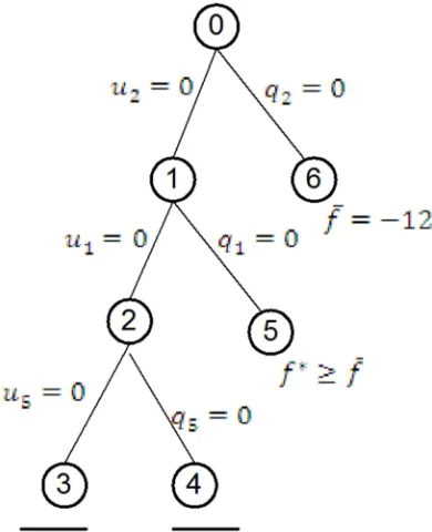
- , so GS 027, Gt ∅, Gu 01,3,4,57 and s 027. In the next two iterations, the algorithm branches - j , -_m, respectively. The index set are GS 02,17, Gt ∅, Gu

03,4,57 and s 02,17. The condition does not satisfy then branching on -_m the sets are G_lS 02,17, G_lt 057, G_lu

03,47 and s_l 02,1,57 this turn out to be infeasible. Then the algorithm backtracks and update the sets G_mS 027, G_mt

017, Gmu 03,4,57 and sm 01,57, a feasible solution is found but fathoming due to optimality backtracking and update the sets G_nS ∅, G_nt 027, G_uu 01,3,4,57 and s_n 027. The optimal solution occurring at the point ∗, H∗

4,4 , -∗_{, -}∗_, -k ∗_{, -l}∗_,

-m

∗ _{0,0.5,0,0,0 with % =12}

and % 8. The full branch and bound tree is shown in Figure 3.

Figure 3. Search tree for the previous Example.

3.3. Fuzzy Approach

While most existing methods are computationally inefficient, a fuzzy approach which uses the membership function of fuzzy set theory as well as multi-objective optimization is developed for solving the BLOP [17, 19, 25]. In this approach, the ULDM specifies preferred values of his/her decision variables and goals with some leeway or tolerance. This information is represented by the use of membership functions of fuzzy set theory and passed to the LLDM. The LLDM should not only optimize his or her objective but also try to satisfy the ULDM's goal and preference as much as possible. He or she realizes that without seriously considering the leader's goal and preference, the proposed solution will very possibly be

rejected and the solution search will be lengthy one. The LLDM then presents his or her solution to the ULDM. If the ULDM agrees to the proposed solution, a solution is reached and it is called a satisfactory solution. If he/she rejects the proposed solution, the ULDM will need to re-evaluate and changes the goals and decisions as well as their leeway or tolerance until a satisfactory solution is reached [17, 19, 25].

Mathematically, the ULDM first solves the following problem:

!" #

$ % , & & &

-./ & *

∈ 0 , ∈ |2 2 3 ., , 4 07 (13)

the solution of which is assumed as {, {, %{ . Independently, the LLDM solves:

!" #

$ % , & & &

-./ & *

∈ 0 , ∈ |2 2 3 ., , 4 0, 7 (14)

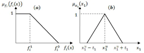
whose solution is assumed to be |, |, %| . These two solutions are then compared. If {, { |, | , then an optimal solution is obtained. However, the two solutions are usually different because of the conflicting nature of the two objectives. The upper-level then reassesses his/her tolerances or vagueness by assuming that the value of { should be "around {" instead of exactly at { with tolerance interval between {= , { and {, { . In other words, the most desirable decision is at { and the most undesirable decision is at the boundary of the interval [17]. Decisions outside the interval are not acceptable. Thus, the following triangular membership functions Figure 4b based on the degree of tolerance of the ULDM can be formulated [17, 19, 25]:

}$

~ • € •

•$ tZ$‚t [, "% {_{= 3 3} { Z$‚S [t$

, "% { _{3 3} {

0, * ( )'"

(15)

The ULDM also must adjust his/her goal by assuming the highest tolerable goal, %u, based on the vagueness of the decentralized organization. Thus, all values of % with

% 3 %{ _{% are absolutely acceptable and all values of %} with % < %u are absolutely unacceptable, and that the preference within % , %u is linearly decreasing as in Figure 4a. Based on this interval of tolerance, we can establish the following linear membership function can now be assumed as [17, 19, 25]:

}?Z% [ ƒ

0, "% % 4 %u ? $ t?„

? t?„ "% %u3 % 3 %

1, "% % 3 %

Figure 4. Membership functions: a) Linear b) Triangular.

The lower-level also reassesses his/her goal by setting the highest tolerable goal %u. Thus, the membership function for the goal of the lower-level can be obtained as follows:

}?Z% [ = ƒ

0, "% % 4 %u ? $ t?„

? t?„ "% %u3 % 3 %

1, "% % 3 %

(17)

The above membership function linearly decreases from 1 at % %|≡ % to 0 at % %u. Let this membership function be represented by † with 0 3 † 3 1, which can be considered as the degree of satisfaction. Similar degrees of satisfactions can also be defined for the upper-level. Let and ‡ represent the degrees of satisfactions for the upper-level's decisions and goal, respectively. In order to satisfy all the degrees of satisfactions, we must find the minimum , ‡ and † simultaneously. Thus, we obtain the following overall satisfactory level [19, 25]:

K !" 0 , ‡, †7 (18) Thus, Equation (18), must be maximized in order to obtain the best degree of satisfaction. Thus, we have the following Multi-Objective Programming (MOP) problem:

!j K !j !" 0 , ‡, †7 -./ & *

2 2 3 .

}$ 4

}?Z% [ 4 ‡

}?Z% [ 4 †

, ‡, † ∈ 0,1 , 4 0, 4 0 (19) substituting the membership functions, for more details see [17, 19, 25], which are represented by Equations (15-17) into Equation (19) we have:

!j K -./ & *

2 2 3 .

= {_{= ⁄ 4 K}

{ _{= ⁄ 4 K}

}?Z% [ % = %u ⁄ % = %u 4 K

}?Z% [ % = %u ⁄ % = %u 4 K

K ∈ 0,1 , 4 0, 4 0 (20) This MOP problem can be solved in many different ways depending on the used algorithm.

Illustrative Example

The numerical example studied in [17] is considered here to illustrate the computational procedure for fuzzy approach.

1 !"#

$ % =2

'( ) * 2 , !"

#

$ % = = 2

-./ & *

∈ _ , `3 = 5 3 15, 3 =3 3 27, 3 4 3 453 21

3 3 30, 4 0, 4 0 e

Solution:

Firstly, solve the ULDM problem as follows:

!"#

$ % =2

-./ & *

∈ _ , `3 = 5 3 15, 3 =3 3 27, 3 4 3 453 21

3 3 30, 4 0, 4 0 e

The solution obtained is {, { 7.5,1.5 with

%{ _{13.5. then solve the lower-level problem as follows:}

!" #

$ % = = 2

-./ & *

∈ _ , `3 = 5 3 15, 3 =3 3 27, 3 4 3 453 21

3 3 30, 4 0, 4 0 e

The solution obtained is |, | 3,9 with %{ 21. As {, { 8 |, | , hence following the above discussion and formulate the membership functions for the upper-level objectives, lower-level objectives and upper-level decision variable. Let the upper-level DM decide { 7.5 and with positive tolerance limits Š 1, one-sided membership function [17, 19, 28].

= 0.085 − 0.0426 + 0.426 ≥ ‡

}?Z% [ =− − 2 − 0_{−21 − 0} = 0.048 + 0.095 ≥ †

}$ = 7.5 + 1 −₁ = 8.5 − ≥

Construct the model in Equation (19), as follows:

!j K -./ & *

0.085 − 0.0426 + 0.426 ≥ K,

0.048 + 0.095 ≥ K,

8.5 − ≥ K,

3 − 5 ≤ 15, 3 − ≤ 21,

3 + ≤ 27, 3 + 4 ≤ 45,

+ 3 ≤ 30, ≥ 0, ≥ 0, K ∈ [0,1]

Thus the satisfactory solution is achieved at ∗, ∗ = 7.313,5.062 with the overall satisfactory level K = 0.8319.

4. Bi-level Multi-Objective Programming

For real world cases, decision making often has multi-objective characteristics, which have been studied in single level decision making, but only a few studies have been conducted in bi-level decision making situations by Wen & Hus [42]. The BL-MODM problem may be formulated as follows [1-3, 11, 31]:

[1 ]

!"#

$ ‹ ,

= !"#

$ Œ% , , % , , … , %6 , •,

'ℎ ) *

[2 , ]

!" #

$ ‹ ,

= !"#

$ Œ% , , % , , … , %6 , •,

-./ & *

∈ = Ž = , ∈ •2 + 2 Œ•M

‘• ., , ≥ 0, . ∈ 6’ (21)

where

%N“ = &N“ + &N“ + ⋯ + &N“ + &N“ + &N“ + ⋯ + &N“ ,

∀ " = 1,2. / = 1,2, … , !N

and where !_N, " = 1,2 are the number of DMj's objective functions, ! is the number of constraints, &_rN“ = Œ&rN“, &rN“, … , &r –

N“ _{• , = 1,2 and &} r –

N“ _{are constants, 2}

N are the

coefficient matrices of size ! × _N, " = 1,2., the control variables = Z , , … , [ and = Z , , … , [, and is the bi-level convex constraints feasible choice set.

Definition 4: For any ∈ _—= 0 | , ∈ 7 given by the ULDM, if the decision variable ∈ _˜= 0 | , ∈ 7 at the lower-level is the non-inferior solution of the LLDM, then , is a feasible solution of the BL-MODM problem [3, 40].

Definition 5: If , is a feasible solution of the BL-MODM problem; no other feasible solution ̅ , ̅ ∈ exist, such that %_“ ̅ , ̅ ≤ %_“ , ; at least one /

/ = 1,2, … , ! is strict inequality, then , is the non-inferior solution of the BL-MODM problem [2, 22, 40].

4.1. FGP Formulation

In BL-MODM problems, if an imperious aspiration level is assigned to each of the objectives %_N“ , " = 1,2, / = 1,2, … , !N, then these fuzzy objectives are termed as fuzzy goals. They are characterized by their associated membership functions by defining the tolerance limits for achievement of their aspired levels. The fuzzy goals of the objectives are

determined by determining individual optimal solutions. The fuzzy goals are then characterized by the associated membership functions which are transformed into fuzzy flexible membership goals by means of introducing over- and under-deviational variables and assigning highest membership value (unity) as aspiration level to each of them. To elicit the membership functions of the decision vectors controlled by the ULDM, the optimal solution of the upper-level MOP problem is separately determined. A relaxation of the decisions is considered to avoid decision deadlock [28, 30, 31].

4.1.1. Construction of Membership Functions

Let ( “, “; %6N_“ , / = 1, … , ! ) and ( “, “; %6N_“ , / = 1, … , ! ) be the optimal solutions of ULDM and LLDM objective functions, respectively, when calculated in isolation. Let š_N“ ≥ %_N“6N be the aspiration level assigned to the "/ ℎ objective %_N“ , . Then, the fuzzy goals [30, 31]:

%N“ , ≲ šN“, " = 1,2, / = 1,2, … , !N, ≅ ∗ (22)

} = ~ €

• 1, "% %N“ 3 šN“

{•ž t?•ž$ ,$

{•ž – •ž , "% šN“3 %N“ 3 -N“ " 1,2, / 1, … , !N

0, "% %N“ 4 -N“

(23)

To build these membership functions, the optimal solution ∗ ∗_, ∗ _{of the upper-level MOP problem [24, 37],} should be determined first. The FGP approach of Mohamed [45], is considered to solve the upper-level MOP problem follows as [28, 31]:

min ¤ ¥ 'S“ ,S“ 6

“M

-./ & *

}? žŒ%“ , • ,t“= ,S“ 1, / 1,2, … , ! ,

2 2 ¦3₄§ ., , 4 0

,t“, ,S“4 0, '" ( ,t“ ,S“ 0, / 1,2, … , ! (24)

where ,t_“, ,S_“, / 1,2, … , ! represent the under- and over-deviations from the aspired levels, and the numerical weights

'S“, / 1,2, … , ! represented as:

'S“ _{{ žt ž}, / 1,2, … , ! (25)

The linear membership functions } ≡ }_$– r for the decision vector Z , , … , [ can be formulated as follows see Figure 5b:

} ≡ }$–Z r[

~ • € •

• $–tŒ$–∗t–¨• –

¨ , "% r∗= r©3 r3 r∗ Œ$–∗_S

– ª_•t$–

–

ª , "% r ∗

3 r₃ r∗

rŠ, 1, … ,

0, * ( )'"

(26)

Figure 5. Membership functions: a) Linear b) Triangular.

4.1.2. FGP Model

In decision making situation, the aim of each DM is to achieve highest membership value (unity) of the associated fuzzy goal in order to obtain the satisfactory solution as [31, 30, 33]:

}?•žŒ%N“ , • ,N“t= ,N“S 1, " 1,2 / 1,2, … , !N (27)

}$–Z r[ ,_rt= ,_rS 1, 1,2, … , (28)

Or equivalently as:

{•ž t?•ž$ ,$ {•ž – •ž ,N“

t_{= ,}

N“S 1, " 1,2 / 1,2, … , !N (29)

$–tŒ$–∗t_–¨•

–¨ ,r

©t_{= ,}

r©S 1, 1,2, … , (30)

Œ$–∗S_–ª•t$– –

ª ,rŠt= ,rŠS 1, 1,2, … , (31)

where ,_rt ,_r©t, ,_rŠt , ,_rS ,_r©S, ,_rŠS , and

,N“t, ,r©t, ,rŠt, ,N“S, ,r©S, ,rŠS4 0 with ,N“t ,N“S 0, ,r©t ,r©S

0, and ,_rŠt ,_rŠS 0 represent the under- and over deviation, respectively, from the aspired levels.

In conventional GP, the under- and/or over-deviational variables are included in the achievement function for minimizing them and also depend up on the type of objective functions to be optimized [31-33]. In this approach, the over-deviational variables for the fuzzy goals of the objective functions, ,_N“S , " 1,2 / 1,2, … , !_N , and the over-deviational and under over-deviational variables for the fuzzy goals of the decision variables, ,_r©t, ,_rŠt, ,_r©Sand ,_rŠS, are required to be minimized to achieve the aspiration level of the fuzzy goals [29].

To assess the relative importance of the fuzzy goals properly, the weighting scheme suggested by Mohamed [45] is used to assign the values to '_N“S, '_r© j , '_rŠ. These values are determined as:

'N“S _{{•žt •ž}, " 1,2 / 1,2, … , !N (32)

'r©

–¨, j , 'r Š

–

ª, 1,2, … , (33)

The FGP model for solving the BL-MODM problem follow as [31-33]:

min ¤ ¥ 'S“ ,S“ ¥ 'S“,S“ 6

“M

¥«'r©Z,r©t ,r©S[ 'rŠZ,rŠt ,rŠS[¬ rM

6

-./ & *

}?žŒ%“ , • + ,t“− ,S“= 1, / = 1,2, … , ! ,

}? žŒ%“ , • + ,t“− ,S“= 1, / = 1,2, … , ! , }$– r + ,rt− ,rS= 1, = 1,2, … ,

2 + 2 ¦≤=_≥§ ., , ≥ 0

,N“t, ,N“S≥ 0, '" ℎ ,N“t ,N“S= 0, " = 1,2 / = 1,2, … , !N

,rt, ,rS≥ 0, '" ℎ ,rt,rS= 0 (34)

The above problem can be rewritten as [31]:

!" ¤ = ¥ 'S“ ,S“+ ¥ 'S“,S“+ 6

“M

¥['r© ,r©t+ ,r©S + 'rŠ ,rŠt+ ,rŠS ] rM

6

“M

-./ & * -“ − %“ ,

- “ − š “ + , “

t _{− ,} “

S _{= 1, / = 1,2, … , ! ,}

-“ − %“ ,

- “ − š“ + , “

t _{− ,} “

S _{= 1, / = 1,2, … , ! ,}

r_{− Z} r∗ − r©[ r© + ,r

©t_{− ,}

r©S= 1, = 1,2, … ,

Z r∗₊

rŠ[ − r

rŠ + ,r

Št_{− ,} r

ŠS_{= 1, = 1,2, … ,}

2 + 2 ¦≤=_≥§ ., , ≥ 0

,N“t, ,N“S≥ 0, '" ℎ ,N“t ,N“S= 0, " = 1,2 / = 1,2, … , !N

,r©S, ,r©t≥ 0, '" ℎ ,r©S ,r©t= 0, = 1,2, … ,

,rŠS, ,rŠt≥ 0, '" ℎ ,rŠS ,rŠt= 0, = 1,2, … , (35)

where ¤ represents the fuzzy achievement function consisting of the weighted over-deviational variables ,_N“S of the fuzzy goals š_N“ and the under-deviational and the over-deviational variables ,_r©t, ,_rŠt, ,_r©S j , ,_rŠS, = 1,2, … , for the fuzzy goals of the decision variables , , … , , where the numerical weights '_N“S, '_r© j , '_rŠ represent the relative importance of achieving the aspired levels of the respective fuzzy goals subject to the constraint set in the decision situation.

4.1.3. The FGP Algorithm for Solving The BL-MODM Problem

Following the above discussion, the proposed FGP algorithm for solving the BL-MOP problem follows as [31]:

Step 1: Calculate the individual maximum and minimum values of each objective function in the two levels under the given constraints.

Step 2: Set the goals and the upper tolerance limits for all the objective function in the two levels.

Step 3: Evaluate the weights '_N“S= 1 -⁄ _N“− š_N“, " = 1,2 / = 1,2, … , !N.

Step 4: Elicit the membership functions }_{? ž}Œ%_“ •, / = 1,2, … , ! , for each of the objective functions in the upper-level.

Step 5: Formulate the Model 24 for the MOP problem of the upper-level.

Step 6: Solve the Model 24 to get ∗= ∗, ∗ , ∗= Œ ∗, ∗, … , ∗•.

Step 7: Set the maximum negative and positive tolerance values on the decision vector

∗_{= Z , , … , [,}

r© j , rŠ, = 1,2, … , .

Step 8: Elicit the membership functions }_$– r for the decision vector = Z , , … , [.

Step 9: Elicit the membership functions }_{? ž}Œ%_“ • , / = 1,2, … , ! , for each of the objective functions in the lower-level.

Step 10: Evaluate '_r©= 1⁄ j , '_r© _rŠ= 1⁄ , =_rŠ 1,2, … , .

Step 11: Formulate the Model 35 for BL-MOLP problem.

Step 12: Solve the Model 35 to get the candidate solution of the BL-MOP problem.

Step 13: If the DM is satisfied with the candidate solution in Step12, go to Step 15, otherwise go to Step 14.

Step 14: Modify the goals and the upper tolerance limits šN“, -N“, " = 1,2 / = 1,2, … , !N for all objective functions in

the two levels, go to Step3.

Step 15: Stop with the satisfactory solution of the BL-MOLP problem.

4.2. The TOPSIS Approach

from the PIS and the longest distance from the NIS) [37, 46, 47].

4.2.1. The TOPSIS Approach for the Upper-Level MOP Problem

Consider the upper-level multi-objective of minimization type problem of the BL-MODM problem as:

!"#

$ ‹ ,

= !"#

$ Œ% , , % , , … , %6 , •,

-./ & *

x ∈ = Ž = , ∈ •2 + 2 ŒM•

‘• ., , ≥ 0, . ∈ 6’ (36)

the TOPSIS approach of Lai et al. [48] that solves single-level MODM problems is considered to solve the upper-level MOP problem. The TOPSIS model formulation of this approach can be follows as:

!" ,®®¯°‚

!j ,®Q¯°‚

-./ & *

∈ = Ž = , ∈ •2 + 2 ŒM•

‘• ., , ≥ 0, . ∈ 6’ (37)

where

,®®¯°‚ = ±∑ '“²³

? ž$ t?∗ž

?´_žt?∗_ž µ ² 6

“M ¶

·

(38)

,®Q¯°‚ = ±∑ '“²³?ž

´_t?ž$

?´_žt? ž ∗ µ

² 6

“M ¶

·

(39)

where %∗_“= !"#

$∈¸ %“

, is the individual positive ideal

solutions, %t_“= !j#

$∈¸ %“

, is the individual negative ideal

solutions and '_“, / = 1, … , ! , is the relative importance (weights) of objectives. Let ‹{∗ = Z%∗, %∗, … , %∗₆ [ and ‹{´

= Z%t_{, %}t_{, … , %} 6

t _{[. Assume that the membership}

functions } and } of the two objective functions are linear between Z,_²{[∗ and Z,_²{[t which are:

Z,®®¯°‚[∗= !"# $∈¸ ,®

®¯°‚

and the solution is ® (40)

Z,®Q¯°‚[∗= !j# $∈¸ ,®

Q¯°‚ _{and the solution is} Q ₍₄₁₎

Z ,®®¯°‚[t= ,®®¯°‚ Q and Z ,®Q¯°‚[t= ,®Q¯°‚ ® (42)

Also, as proposed in [34, 37] by A. Baky that Z ,_®®¯°‚[t and Z ,_®Q¯°‚[t can be taken as Z ,_®®¯°‚[t= !j#

$∈¸ ,® ®¯°‚

and Z ,_®Q¯°‚[t= !"#

$∈¸ ,® Q¯°‚

, respectively. Let ,_®{∗ =

ŒZ ,®®¯°‚[∗, Z ,®Q¯°‚[∗ • and ,®{´= ZZ ,®®¯°‚[t, Z ,®Q¯°‚[t [.

Thus If we assume that the membership functions } ≡ }_¹ºº»¼‚ and } ≡ }_¹º½»¼‚ then it can be obtained as:

} =

~ • € •

• 1, "% ,®®¯°‚ < Z ,®®¯°‚[∗

1 −¹ºº»¼‚$ tŒ ¹ºº»¼‚•∗ Z ¹ºº»¼‚[´tZ ¹ºº»¼‚[∗, "% Z ,®

®¯°‚

[∗≤ ,®®¯°‚ ≤ Z ,®®¯°‚[t

0, "% Z ,®®¯°‚[t< ,®®¯°‚

(43)

} =

~ • € •

• 1, "% ,®Q¯°‚ > Z ,®Q¯°‚[∗

1 − Œ ¹º½»¼‚•∗t ¹º½»¼‚ $

Œ ¹_º½»¼‚•∗tŒ ¹_º½»¼‚•´, "% Z ,®

Q¯°‚_[t_{≤ ,} ®

Q¯°‚ _{≤ Z ,}

®Q¯°‚[∗

0, "% ,®Q¯°‚ < Z ,®Q¯°‚[t

(44)

Thus, resolve the model in Equation (37) and obtaining the satisfying decision of the upper-level MOP problem,

∗₌ ∗_, ∗ _{, by solving the following problem:}

}¿ = !j#

$∈¸ B!" Z} , } [D

(45)

Thus, by introducing a variable = !" Z} , } [, model of Equation (37) is equivalent to the form of

Tchebycheff model, for more details see [48, 49], which is equivalent to the following model:

!j -./ & *

} ≥ ,

∈ = Ž = , ∈ •2 + 2 Œ•M

‘• ., , ≥ 0, . ∈ 6’ (46)

where is the overall satisfactory level for both criteria of the shortest distance from the PIS and the farthest distance from the NIS. According to this concept, the linear membership functions for each of the components of decision vector ∗= Œ ∗, ∗, … , ∗• controlled by the ULDM can be formulated as [34]:

}_$– r =

~ • € •

• $–tŒ$–∗t–¨• –¨ , "%

r∗

− r©≤ r≤ r∗ Œ$–∗S_–ª•t$–

–ª , "%

r∗ _≤ r_≤ r∗₊

rŠ, = 1, … ,

0, * ℎ )'"

(47)

4.2.2. The TOPSIS Approach for the BL-MODM Problem

In order to obtain a compromise solution (satisfactory solution) to the BL-MODM problem using the TOPSIS approach, the distance function from the positive and the negative ideal solution, ,_®®¯°À,_®Q¯°À, as follows [34, 37]:

,®®¯°À = ±∑ '²“³

?_ž $ t?∗_ž ?´_žt?∗_ž µ

²

+ ∑ '²“³

? _ž$ t?∗_ž ?´_žt?∗_ž µ

² 6

“M 6

“M ¶

·

(48)

,®Q¯°À = ±∑ '²“³?ž

´_t?ž$

?´_žt? ž ∗ µ

² 6

“M + ∑ '²“³?ž

´_{t? ž$}

?´_žt? ž ∗ µ

² 6

“M ¶

·

(49)

where '_r, = 1,2, … , ! + ! are the relative importance of objectives in both levels. %_N“∗ = !"#

$∈¸ %N“ , %N“ t₌

!j#

$∈¸ %N“ , " = 1,2, / = 1,2, … , !N

, and Á = 1,2, … , ∞. Let

‹∗_{= Z%}∗_{, %}∗_{, … , %} 6

∗ _{, %}∗_{, %}∗_{, … , %} 6

∗ _{[ , and ‹}t₌

Z%t_{, %}t_{, … , %} 6

t _{, %}t_{, %}t_{, … , %} 6 t _[.

In order to obtain a compromise solutions, the problem is

transferred into the following bi-objective problem with two commensurable (but often conflicting) objectives [46-48, 50]:

!" ,®®¯°À

!j ,®Q¯°À

-./ & *

∈ = Ž = , ∈ •2 + 2 ŒM•

‘• ., , ≥ 0, . ∈ 6’ (50)

Assume that the membership functions }_k ≡ }_¹ º

º»¼À and }l ≡ }_¹

º

½»¼À can be obtained as follows [48]:

}k =

~ • € •

• 1 "% ,®®¯°À > Œ ,®®¯°À• ∗

1 − ¹ºº»¼À$ t ¹ºº»¼Àà ∗

Œ ¹_ºº»¼À•´tŒ ¹_ºº»¼À•∗ "% Œ ,®

®¯°À_•∗_{≤ ,} ®

®¯°À _{≤ Œ ,}

®®¯°À• t

0 "% Œ ,®®¯°À• t

< ,®®¯°À

(51)

}l =

~ • € •

• 1 "% ,®Q¯°À > Œ ,®Q¯°À• ∗

1 −  ¹º½»¼Àà ∗

t ¹_º½»¼À$

Œ ¹_º½»¼À•∗tŒ ¹_º½»¼À•´ "% Œ ,® Q¯°À

•t≤ ,®Q¯°À ≤ Œ ,®Q¯°À• ∗

0 "% ,®Q¯°À < Œ ,®Q¯°À• t

(52)

To obtain the compromise solution ∗= ∗, ∗ , of model in Equation (48-49) Applying the max-min decision model of Bellman and Zadeh [43] as follows:

}¿ = !j#

$∈¸ B!" Z}k , }l [D

(53)

!j † -./ & *

}k ≥ †,

}l ≥ †, † ∈ [0,1],

∈ = Ž = , ∈ •2 + 2 ŒM•

‘• ., , ≥ 0, . ∈ 6’ (54)

where † is the satisfactory level for both criteria. It is well known that if the optimal solution of the model in Equation (54) is the vector †, ∗, ∗ .

The final proposed model can be obtained as [34, 37]:

!j † -./ & *

1 −,®

®¯°À

− Œ ,®®¯°À• ∗

Z ,®®¯°À[ t

− Z ,®®¯°À[ ∗≥ †,

1 − Œ ,®

Q¯°À

•∗− ,®Q¯°À

Z ,®Q¯°À[∗− Z ,®Q¯°À[t

≥ †,

r_{− Z} r∗ − r©[

r© ≥ †,

Z r∗

+ rŠ[ − r

rŠ ≥ †, = 1,2, … , , j , † ∈ [0, 1]

∈ = Ž = , ∈ •2 + 2 ŒM•

‘• ., , ≥ 0, . ∈ 6’ (55)

4.2.3. The TOPSIS Algorithm for the BL-MOP Problem

Following the above discussion, the algorithm for the proposed TOPSIS approach for solving the BL-MODM problem is given as follows [34]:

Step 1: Calculate the individual maximum and minimum values of all the objective functions in the two levels under the system constraints.

Step 2: Construct the PIS payoff table of the ULDM problem 36 and obtain ‹{∗= Z%∗, %∗, … , %∗₆ [, the individual positive ideal solutions.

Step 3: Construct the NIS payoff table of the ULDM problem 37 and obtain ‹{´= Z%t, %t, … , %t₆ [, the individual negative ideal solutions.

Step 4: Use Eq. 38 to construct ,_®®¯°‚ and ,_®Q¯°‚ . Step 5: Ask the DM to select p, 0Á = 1,2, … , ∞7. Step 6: Construct the payoff table of problem 39 and obtain Z,_²{[∗ and Z,_²{[t.

Step 7: Elicit the membership functions }_¹

ºº»¼‚ and }_¹º½»¼‚ .

Step 8: Formulate the model 46 for the ULDM problem. Step 9: Solve model 46 to get ∗= ∗, ∗ , j , ∗= Œ ∗, ∗, … , ∗•.

Step 10: Set the maximum negative and positive tolerance values on the decision vector ∗= Œ ∗, ∗, … , ∗• , _r© and

rŠ, = 1,2, … , .

Step 11: Construct the PIS and NIS payoff table of the BL-MODM problem.

Step 12: Use Eq. 48 − 49 to construct ,_®®¯°À and ,®Q¯°À , respectively.

Step 13: Construct the payoff table of problem 50 and

obtain Z,_²Ä[∗ and Z,_²Ä[t.

Step 14: Elicit the membership functions }

¹_ºº»¼À and

}_¹

º½»¼À .

Step 15: Elicit the membership functions Eq. (47) }$– r , = 1,2, … , .

Step 16: Formulate the model 55 for the BL-MODM problem.

Step 17: Solve model 55 to get ∗= ∗, ∗ .

Step 18: If the DM is satisfied with the candidate solution in Step 17, go to Step 20, else go to Step 19.

Step 19: Modify the maximum negative and positive tolerance values on the decision vector

∗_{= Œ} ∗_, ∗_{, … ,} ∗_•,

r© and rŠ, = 1,2, … , , go to

Step 15.

Step 20: Stop with a satisfactory solution, ∗= ∗, ∗ , to the BL-MODM problem.

5. Conclusion

In this article we present a survey on different approaches for solving BLOP. Some basic approaches for solving the BLOP such as; vertex enumeration, branch and bound algorithm, Karush Kuhn-Tucker (KKT) transformation, fuzzy programming approach are exhibited. Finally, formulation of the BL-MODM problem and recently developed approaches, such as; FGP and TOPSIS approach, for solving such problem are presented. Several open points for research in the area of BLOP, from our point of view, to be studied in the future. Some of these points are given in the following:

1.Interactive approach for BLOP with random rough parameters.

optimization algorithm.

3.Multi-level linear fractional optimization problem with rough environment via FGP.

Conflict of Interest

The authors declare that they have no conflict of interest.

References

[1] Osman, M. A., Emam, O. E. and El Sayed, M. A., Solving Multi-level Multi-objective Fractional Programming Problems with Fuzzy Demands via FGP Approach, International Journal of Applied and Computational Mathematics, 4 (1) (2018), 4-41. [2] Osman, M. A., Emam, O. E. and El Sayed, M. A., On

parametric multi-level multi-objective fractional programming problems with fuzziness in the constraints, British Journal of Mathematics and Computer science, 18 (5) (2016), 1-19. [3] Osman, M. A., Emam, O. E. and El Sayed, M. A., Interactive

Approach for Multi-Level Multi-Objective Fractional Programming Problems with Fuzzy Parameters, Beni-Suef journal of basic and applied sciences, 7 (1) (2018),139-149. [4] Osman, M. S., Emam, O. E., Raslan, K. R. and Farahat, F. A.,

Solving Fully Rough Interval Multi-level Multi-objective linear Fractional Programming Problems via FGP, Journal of Statistics Applications & Probability, 7 (1) (2018), 115-126. [5] Osman, M. S., Emam, O. E., Raslan, K. R. and Farahat, F. A.,

Solving Multi-level Multi-objective Fractional Programming Problem with Rough Intervals in the Objective Functions, British Journal of Mathematics & Computer Science, 21 (2) (2017), 1-17.

[6] Osman, M. S., Emam, O. E., Raslan, K. R. and Farahat, F. A., Solving bi-level multi-objective quadratic fractional programming problems in rough environment through FGP approach, Journal of Abstract and Computational Mathematics, 3 (1) (2018), 6-21.

[7] Osman, M. A., Emam, O. E. and El Sayed, M. A., Stochastic Fuzzy Multi-level Multi-objective Fractional Programming Problem: A FGP Approach, OPSEARCH, 54 (4) (2017), 816-840. [8] Osman, M. A., Emam, O. E. and El Sayed, M. A., Multi-level Multi-objective Quadratic Fractional Programming Problem with Fuzzy Parameters: A FGP Approach, Asian Research Journal of Mathematics, 5 (3) (2017), 1-19.

[9] Ranarahu, N., Dash, J. K., and Acharya, S., Multi-objective bi-level fuzzy probabilistic programming problem, OPSEARCH 54 (3) (2017), 475–504.

[10] El-Sobky, B., and Abo-Elnaga, Y., A penalty method with trust-region mechanism for nonlinear bi-level optimization problem. Journal of Computational and Applied Mathematics, 340 (2018), 360-374.

[11] Gao, Y., "Bi-level decision making with fuzzy sets and particle swarm optimization", Ph. D. Faculty of Engineering and Information Technology, University of Technology, Sydney, UTS Australia, (2010).

[12] Candler, W., and Townsley, R., "A linear bi-level programming problem", Computers & Operations Research 9, (1982) 59-76.

[13] Amat-Fortuny, J., and McCarl, B. "A representation and economic interpretation of two-level programming problem", Journal of the Operation Research Society, 32. (1981) 783-792.

[14] Bialas, W. F., and Karwan, M. H., "Two-level linear programming", Management Science, vol. 30, no. 8, pp. (1984) 1004-1020.

[15] Bialas, W. F., and Karwan, M. H., "On two-level optimization", IEEE Transactions on Automatic Control, AC. 26 No. 1, pp. (1982) 211-214.

[16] Ayed, O. B., "Bi-level linear programming", Computers and operations research, Vol. 20 No. 5 pp. (1993) 485-501. [17] Lee, E. S., and Shih, Hsu-shih, "Fuzzy and multi-level

decision making an interactive computational approach", Springer-Verlag, London limited, (2001).

[18] Lai, Y. J., "Hierarchical Optimization: A satisfactory solution", Fuzzy Sets and Systems 77, (1996) 321-335.

[19] Shih, H. S., Lai, Y. J., and Lee, E. S., "Fuzzy approach for multi-level programming problems", Computers & Operations Research, 23 (1996) 73-91.

[20] Shih, H. S., and Lee, E. S., "Compensatory fuzzy multiple level decision making", Fuzzy Sets and Systems 14, 2000 71-87. [21] Sakawa, M., Nishizaki, I., and Uemura, Y., "Interactive fuzzy

programming for two-level linear fractional programming problems with fuzzy parameters". Fuzzy Sets and Systems, 115 (2000) 93- 103.

[22] Sakawa, M., and Nishizaki, I., "Interactive fuzzy programming for decentralized two-level linear programming problems", Fuzzy Sets and Systems, 125 (2002) 301-315.

[23] Shi, X., and Xia, H., "Interactive bi-level multi-objective decision making", Journal of the Operational Research Society, Vol. 48 pp. (1997) 943-949.

[24] Abo-Sinna, Mahmoud A., "A bi-level non- linear multi-objective decision making under fuzziness", OPSEARCH, 38 (5) (2001) 484-495.

[25] Osman, M. S., Abo–Sinna, M. A., Amer, A. H., and Emam, O. E., "A Multi-level non-linear multi-objective decision making under fuzziness", Journal of Applied Mathematics and Computation Vol. 153 pp. (2004) 239-252.

[26] Abo-Sinna, Mahmoud A., and Baky, I. A., "Interactive balance space approach for solving bi-level multi-objective programming problems", Advances in modeling and Analysis, B 49 (3-4) (2006) 43- 62.

[27] Zhang, G., Lu, J., and Dillon, T., "Decentralized multi-objective bi-level decision making with fuzzy demands", Knowledge-Based System, 20 (5)(2007), 495-507.

[28] Moitra, B. N., and Pal, B. B., "A fuzzy goal programming approach for solving bi-level programming problems", in: N. R. Pal and M. Sugeno, (Eds.), AFSS (2002), LNAI 2275, PP. 91-98, Springer, Berlin, Germany.

[30] Pramanik, S., and Roy, T. K., "Fuzzy goal programming approach to multi-level programming problems", European Journal of Operational Research, vol. 176, no. 2, pp (2007) 1151-1166.

[31] Baky, I. A., "Fuzzy goal programming algorithm for solving decentralized bi-level multi-objective programming problems", Fuzzy Sets and Systems, vol. 160, no. 18, pp. (2009) 2701-2713.

[32] Baky, I. A., "Solving multi-level multi-objective linear programming problems through fuzzy goal programming approach", Applied Mathematical Modeling, 34 (9) (2010) 2377-2387.

[33] Baky, I. A., Eid, M. H., and El-Sayed, M. A., "Bi-level Multi-objective Programming Problem with Fuzzy Demands: A Fuzzy Goal Programming Algorithm", OPSEARCH, 51 (2) (2014) 280-296.

[34] Baky, I. A., and Abo-Sinna, M. A., "TOPSIS for bi-level MODM problems", Applied Mathematical Modeling, 37 (2013), 1004-1015.

[35] Chen L. H. and Chen H. H., A two-phase fuzzy approach for solving multi-level decision-making problems, Knowledge-Based Systems 76 (2015) 189-199.

[36] Youness, E. A., Emam, O. E. and Hafez, M. S., Fuzzy bi-level multi-objective fractional integer programming. Appllied Mathimatics and Information Science. 8 (6) (2014), 2857– 2863.

[37] Baky, I. A. and El-Sayed, M. A., Bi-level multi-objective programming problems with fuzzy parameters: modified TOPSIS approach, International Journal of Management and Fuzzy Systems, 2 (5) (2014), 38-50.

[38] Lachhwani K., On solving multi-level multi objective linear programming problems through fuzzy goal programming approach, OPSEARCH 51 (4) (2014), 624–637.

[39] Ren, A., A novel method for solving the fully fuzzy bi-level linear programming problem. Math. Probl. Eng. 2 (2015), 1– 11.

[40] Emam, O. E., "On Multi-level Non-linear programming problems", Ph. D. Dissertation, Mathematics Department, Faculty of Science, Helwan University, Egypt, (2004). [41] Wen, U. P., and Lin, S. F., "Finding an efficient solution to

linear bi-level programming problem: an efficient approach", Journal of Global Optimization, Vol. 8 pp. (1996) 295-306. [42] Wen, U. P., and Hsu, S. T., "Linear bi-level programming

problems", Journal of Operations Research Society, Vol. (42) No. 2 pp. (1991) 125-133.

[43] Bellman, R. E., and Zadeh, L. A., "Decision making in a fuzzy environment", Management Science, 17 (1970) 141-164. [44] Shi Chenggen, Lu Jie, and Zhang, G., "An extended

Kuhn-Tucker approach for linear bi-level programming", Journal of Applied Mathematics and Computation 162 (2005) 51-63. [45] Mohamed, R. H., "The relationship between goal

programming and fuzzy programming", Fuzzy Sets and Systems, 89 (1997) 215-222.

[46] Abo-Sinna, Mahmoud A., and Amer, A. H., "Extensions of TOPSIS for multi-objective large-scale nonlinear programming problems", Journal of Applied Mathematics and Computation, 162 (2000) 243-256.

[47] Abo-Sinna, Mahmoud A., "Extensions of the TOPSIS for multi-objective dynamic programming problems under fuzziness", Advances in Modeling and Analysis, B 43 (4) (2000) 1-24.

[48] Lai, Y. J., Liu, T. J., and Hwang, C. L., "TOPSIS for MODM", European Journal of Operational Research. 76 (1994) 486-500.

[49] Lai, Y. J., and Hwang, C. L., "A new approach to some possibilistic linear programming problems", European Journal of Operational Research. 176 (2006) 1151-1166.