R E S E A R C H
Open Access
Spatial and temporal analysis of beta
diversity in the Barro Colorado Island forest
dynamics plot, Panama
Pierre Legendre
1*and Richard Condit
2,3Abstract
Background:Ecologists are interested in assessing the spatial and temporal variation in ecological surveys repeated over time. This paper compares the 1985 and 2015 surveys of the Barro Colorado Forest Dynamics plot (BCI), Panama, divided into 1250 (20 m × 20 m) quadrats.
Methods, spatial analysis:Total beta diversity was measured as the total variance of the Hellinger-transformed community data throughout the BCI plot. Total beta was partitioned into contributions of individual sites (LCBD indices), which were tested for significance and mapped.
Results, spatial analysis: LCBD indices indicated the sites with exceptional community composition. In 1985, they were mostly found in the swamp habitat. In the 2015 survey, none of the swamp quadrats had significant LCBDs. What happened to the tree community in the interval?
Methods, temporal analysis:The dissimilarity in community composition in each quadrat was measured between time 1 (1985) and time 2 (2015). Temporal Beta Indices (TBI) were computed from abundance and presence-absence data and tested for significance. TBI indices can be decomposed intoB= species (or abundances-per-species) losses
and C= species (or abundances-per-species) gains. B-C plots were produced; they display visually the relative
importance of the loss and gain components, through time, across the sites.
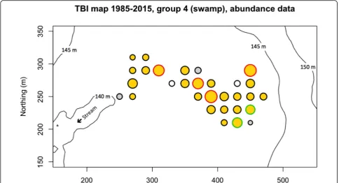
Results, temporal analysis: In BCI, quadrats with significant TBI indices were found in the swamp area, which is shrinking in importance due to changes to the local climate. A published habitat classification divided the BCI forest plot into six habitat zones. Graphs of theBandCcomponents were produced for each habitat group. Group 4 (the swamp) was dominated by species (and abundances-per-species) gains whereas the five other habitat groups were dominated by losses, some groups more than others.
Conclusions:We identified the species that had changed the most in abundances in the swamp between T1 and T2. This analysis supported the hypothesis that the swamp is drying out and is invaded by species from the surrounding
area. Analysis of the B and C components of temporal beta diversity bring us to the heart of the mechanisms
of community change through time: losses (B) and gains (C) of species, losses and gains of individuals of various species. TBI analysis is especially interesting in species-rich communities where we cannot examine the changes in every species individually.
Keywords: Beta diversity, B-C plots, BCI forest dynamics plot, Space-time analysis, Temporal beta diversity
* Correspondence:[email protected]
1Département de sciences biologiques, Université de Montréal, C.P. 6128,
succursale Centre-ville, Montréal, Québec H3C 3J7, Canada Full list of author information is available at the end of the article
Background
Whittaker (1972) defined beta diversity as spatial differ-entiation, or the variation in species composition among sites within a region of interest. Different ways of meas-uring beta have been proposed by Whittaker himself and by other authors. Several authors have argued that the variance of a community composition data table (sites x species) is an appropriate measure of beta diversity across the sites (Koleff et al.2003; Legendre et al.2005; Anderson et al. 2011). It has also been shown that the total variance can be computed from a dissimilarity matrix D obtained from an appropriately chosen dissimi-larity indexD. Legendre & De Cáceres (2013) described properties of dissimilarity indices that are necessary for beta diversity studies and identified 11 indices that were appropriate for such studies; two more indices were added to that list by Legendre (2014) and Legendre & Borcard (2018).
The concept of beta diversity can be extended to time. It was called temporal beta diversity by Legendre and Gau-thier (2014) and by Shimadzu et al. (2015). Temporal beta variation can be the result of gradual or abrupt changes in environmental conditions, including man-induced alter-ations such as the ongoing worldwide climate warming. Re-search on temporal variation in communities is conducted, for example, at hundreds of research sites affiliated to the International Long Term Ecological Research (ILTER) net-work (https://www.ilter.network), and in the dynamics for-est plots affiliated with the Forfor-est Global Earth Observatory (ForestGEO; seehttps://forestgeo.si.edu/).
A statistical method for the analysis of temporal beta di-versity has recently been described by Legendre (2019). The objective is to compare observations made during two separate surveys through time, involving several sites. The method has two distinct parts: (1) estimate the change in each geographic sampling unit (site) between time 1 (abbreviated T1) and time 2 (T2), using an appro-priate dissimilarity index, called a temporal beta-diversity index (TBI), and test the significance of that change to identify the sites where the change has been exceptionally important; these sites may be worth examining to identify the causes of the differences. And (2) partition the dissimi-larity information into finer indices of losses and gains of species, or of abundances-per-species, which may tell us something about the processes at work in the system, which may have generated these changes. Applications of that method have already been published in palaeoecology (Winegardner et al. 2017) and in the study of freshwater (Kuczynski et al. 2018) and marine animal communities (Legendre & Salvat2015). Three other ecological applica-tions of the method are presented in the Legendre (2019) paper.
The TBI method will be illustrated in this paper by an analysis of a 50-ha permanent forest dynamics plot. The
precise questions we will try to answer about the plot are the following: (1) Is there a region in the plot where the changes in community composition have been especially important between 1985 and 2015? (2) If there is such an area, what happened in the community? Was the change characterized by species (or abundances-per-species) losses or gains? (3) And finally, what are the species that changed more strongly? If the change was mostly a gain of species, was this the result of a migration or an invasion, and where did these species come from?
Methods Plot and censuses
The Barro Colorado Forest Dynamics plot (BCI) in Panama was established in 1981 by Robin Foster and Stephen Hubbell (Hubbell and Foster 1983). Data from this plot have been used in many scientific papers, in-cluding a recent one by Condit et al. (2017b) in this journal, where the plot and the survey method are de-scribed. Some statistics about the plot are provided in Table1. This 50-ha plot has been subjected to 8 detailed surveys since its inception: in 1982+, 1985, 1990, 1995, 2000, 2005, 2010 and 2015. The present paper is the first application of the TBI method of analysis to the data of a permanent forest dynamics plot. It will serve as a model for the analysis of other forest plots. At the mo-ment, the ForestGEO network includes some 70 such forest plots throughout the world. The census data can be downloaded from Condit et al. (2012,2017a).
The BCI data were divided into 1250 quadrats of size (20 m × 20 m) before analysis; this was deemed the most appropriate scale of study to answer the ecological
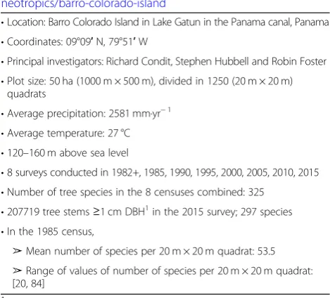
Table 1Basic information about the Barro Colorado Forest Dynamics plot (BCI) in Panama. For more information, see Condit et al. (2017b) andhttps://forestgeo.si.edu/sites/ neotropics/barro-colorado-island
•Location: Barro Colorado Island in Lake Gatun in the Panama canal, Panama
•Coordinates: 09°09′N, 79°51′W
•Principal investigators: Richard Condit, Stephen Hubbell and Robin Foster
•Plot size: 50 ha (1000 m × 500 m), divided in 1250 (20 m × 20 m) quadrats
•Average precipitation: 2581 mm·yr−1
•Average temperature: 27 °C
•120–160 m above sea level
•8 surveys conducted in 1982+, 1985, 1990, 1995, 2000, 2005, 2010, 2015
•Number of tree species in the 8 censuses combined: 325
•207719 tree stems≥1 cm DBH1in the 2015 survey; 297 species
•In the 1985 census,
➢Mean number of species per 20 m × 20 m quadrat: 53.5 ➢Range of values of number of species per 20 m × 20 m quadrat: [20, 84]
1
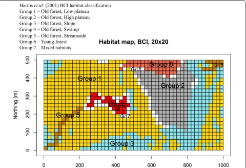
questions addressed in the present paper, which com-pares the surveys conducted in 1985 and 2015. The union of the species identified in the 1985 and 2015 sur-veys was 328. Figure1shows a habitat classification map of the BCI forest proposed by Harms et al. (2001). Statistical methods for spatial analysis
A preliminary spatial analysis of the forest plot will be done first. Total beta diversity, computed as the total vari-ance of the Hellinger-transformed multivariate commu-nity composition data throughout the BCI plot, will be partitioned into Local Contributions to Beta Diversity
(LCBD indices) in order to determine where the quadrats are found that are the most different from the multivariate centroid of all quadrats. LCBD indices can be tested for significance. The computation method and interpretation have been described by Legendre & De Cáceres (2013). Calculations were done using the beta.div function of the
adespatialpackage in R (Dray et al.2019). Statistical methods for temporal analysis
The main part of the paper will consist in a temporal beta diversity analysis focussing on the three questions
listed at the end of the Introduction. The methods are the following.
Space-time interaction
For censuses repeated through time, as it is the case in Forest Dynamics Plots, the interaction between space (S) and time (T) is of great interest. A significant interaction would indicate that the spatial structure of the response data has changed through time, and conversely, that the temporal variations differed significantly among the sites (quadrats), indicating, for example, an effect of climate change. The space-time interaction (STI) can be tested on univariate or multivariate data using the method pro-posed by Legendre et al. (2010), despite the lack of repli-cated observations. That method is implemented in function stimodels() of the adespatial package in R (Dray et al. 2019). The community data were trans-formed using the Hellinger transformation (Legendre & Gallagher2001) before this analysis.
Temporal beta diversity indices (TBI)
The dissimilarity in community composition was mea-sured for each of the 1250 quadrats of the BCI plot
between time 1 (T1 = 1985 survey) and time 2 (T2 = 2015 survey). The analysis was repeated separately for the 30 quadrats of group 4 (the swamp).
The index used for community composition data will be the percentage difference (or % difference; Odum 1950), also known as the Bray-Curtis index. The Sørensen index will be used for occurrence (presence-absence) data; this is the binary form of the percentage difference index (Legendre & Legendre 2012). In the context of a comparison through time, these indices are called
Temporal Beta Indices (TBI). These indices can be
tested for significance, as shown in Legendre (2019). Each index, which compares data from a quadrat at T1 and T2, is composed of two parts: B= species (or abundances-per-species) losses and C= species (or abundances-per-species) gains.
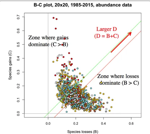
The B and C statistics will be used to produce B-C plots, with B (losses per quadrat) in the abscissa andC
(gains per quadrat) in the ordinate, as described in Le-gendre (2019). B-C plots display visually the relative im-portance of the loss and gain processes in a study area, informing researchers about details of the processes of biodiversity losses and gains across the sites, through time, in space-time surveys. B-C plots will be shown for the whole BCI forest plot and for six separate habitats within the plot.
The mean of the differences between theBand C sta-tistics is also computed across all sites in a study. A positive value of (C – B) indicates that the study area was dominated by gains, whereas a negative value indi-cates overall losses of species or abundances-per-species. The (C–B) difference across all quadrats was tested for significance using a pairedt-test computed for theCand
Bstatistics from all sites in the study. The calculation in-volves the mean of the differences (C/den–B/den) at all sites; in the present study, den was the denominator of Odum’s percentage difference index, (2A+B+C).
The calculations are implemented in the TBI() and plot.TBI() functions, available in the R package adespa-tial(Dray et al.2019).
Changes in species composition from T1 to T2
In order to understand in more detail the demographic changes at BCI in the quadrats of the swamp habitat in the 1985–2015 interval, we analysed the changes in the 209 species found in the swamp from 1985 to 2015, across its 30 quadrats, using paired t-tests. The tests were carried out with 9999 random permutations of the values, in each quadrat, between T1 and T2. A Holm (1979) correction for multiple testing (209 simultaneous tests had been conducted) was applied to the computed
p-values. The calculations are implemented in function tpaired.krandtest.Rpaired.t.test.spec(), available in the R packageadespatial(Dray et al.2019).
Results
Preliminary spatial analysis
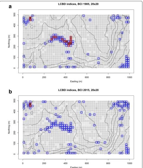
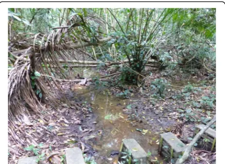
The quadrats that have high and significant LCBD indices (quadrats with red rims in Fig. 2a) are the most different in species composition from a hypothetical quadrat found at the multivariate centroid of a PCA ordination. The sig-nificant quadrats are found mostly in the central portion of the map, in an area called the swampby Harms et al. (2001). This is an old forest habitat where water accumu-lates during the rainy season and which harbours a differ-ent flora than the rest of the BCI plot. The oil palm,Elaeis oleifera(Kunth) Cortés, is a conspicuous indicator species of the swamp community (Plate1).
Comparison of Fig. 2a and b shows that no quadrat with a red rim remained in the swamp area in the 2015 survey data. This preliminary analysis allows us to ask a new question: Why is it that quadrats with highly significant LCBD indices are no longer found in the swamp in 2015?
Temporal beta diversity analysis
The number of stems declined substantially during that period 1985–2015 (Fig. 3): there was a net loss of 35,638 stems between 1990 and 2005, representing about 15% of the stems that were found in 1990 (244,015 stems).
Space-time interaction
A significant space-time interaction was reported across 4 censuses (from 1982 to 83 to 1995) by Legendre et al. (2010) for the whole community of 315 species in the (20 m × 20 m) quadrats and for 43% of the individual species tested separately.
We checked that this was still the case for the seven censuses conducted between 1985 and 2015. Indeed, a significant space-time interaction was detected for the (20 m × 20 m) quadrats. This significant interaction means that the spatial structure of the multivariate data has changed significantly among the censuses. We will now study these differences in more detail between cen-suses #2 (1985) and #8 (2015) for the whole plot, then for each habitat type separately, using temporal beta di-versity indices and B-C plots.
Temporal beta diversity indices (TBI)
a
b
quadrats had the highest TBI values among the 1250 quadrats of the BCI forest plot, indicating that they were the most different in composition between the 1985 and 2015 surveys.
The mean of the differences between of C/den
(losses) and B/den (gains) over the entire BCI forest plot was negative, indicating dominance of losses across all 1250 quadrats (detailed output file not shown). The test of significance of that difference was highly signifi-cant. In the separate analysis of the group 4 data (de-tailed output file in Additional file1: Appendix S1), this
same comparison showed a positive difference of the mean of (C/den–B/den) over the swamp quadrats, in-dicating that gains of individuals-per-species had dominated group 4 in the time interval under study; see output element $t.test_B.C in Additional file 1: Appendix S1. The test of significance of that difference was also highly significant.
B-C plots
A first B-C plot is shown in Fig.5for the 1250 quadrats of the BCI forest. In this overall plot, the green line is above the red line, materializing in a figure the statistical result found in the previous subsection: losses of abundances-per-species dominated the changes in the entire BCI forest from 1985 to 2015.
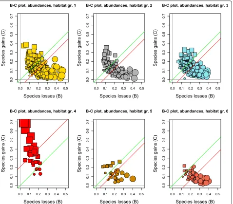
Separate B-C plots were then produced for habitat groups 1 to 6, abundance data (Fig. 6). In all habitat types except group 4, the green line is above the red line, indicating that species losses dominated gains. In group 4 (the swamp), however, the red line is above the green line, indicating that gains dominated losses in this habi-tat. The same result was found when analysing occur-rence data in the 6 habitat types; see Supporting information, Additional file1: Appendix S2.
Changes in species composition from T1 to T2
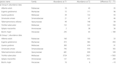
The paired t-tests computed separately for the 209 spe-cies of group 4 (the swamp) over its 30 quadrats showed that 7 species had significant increases in abundances (number of stems) in these quadrats from 1985 to 2015 (Table 2a) whereas one, Bactris major, decreased in
Fig. 3Number of tree stems in the BCI forest plot recorded during 7 surveys from 1985 to 2015
abundance. The species that increased in abundances also increased in occurrences, and conversely.
For comparison, six of the seven species that increased in group 4 also increased in abundances in group 1 (Table 2b). Only Trichilia tuberculata decreased in group 1 while increasing in group 4.
Of course, these 209 individual tests are not proper paired t-tests of comparison of means because the data are from contiguous quadrats, hence they are strongly autocorrelated. Yet, the tests allowed us to identify the species where the differences in abundances between T1 and T2 were the strongest in group 4 (Table 2a). B.
major decreased in abundance and in occurrences in
both habitats.
The species we were looking for here are those that changed the most in the T1-T2 interval. This is different from the search for indicator species of the six habitat groups. For example, we mentioned above that the oil palm, Elaeis oleifera, was a most conspicuous indicator species of the swamp habitat. This species has not no-ticeably changed in abundance in the swamp between 1985 and 2015, going from 16 to 17 individuals.
Discussion and conclusion
Results of the individual analyses presented in the previ-ous section combine into a coherent story of what hap-pened in the BCI forest plot.
Preliminary spatial analysis
Analysis of the local contributions to beta diversity (LCBD) at the quadrat level showed that in 1985, the swamp area (habitat group 4) had a highly distinctive community, with many quadrats significantly different from the other habitat types of the BCI plot. In 2015, this community was still different in composition but the im-portance of the difference had subsided. This observation called for a more detailed analysis of the difference be-tween the 1985 and 2015 surveys in the swamp area.
Temporal beta diversity analysis
At BCI, the period 1982–1992 included several extreme dry seasons; since then, there have been few such drought events. High tree growth rates and death rates were observed during the drought but not since then (Condit et al.,2017b). A simple indicative statistic is the loss of 36,761 tree stems between 1990 and 2010, or 15% of the stems surveyed in 1990 (Fig.3).
The annual amount of rain has a strong influence on tropical forest composition. It determines the height of the water table and has consequences on many other en-vironmental factors. Changes in soil wetness and dryness is an important factor determining changes in species composition in the long run, considering the fact that tropical trees are long-lived. However, one cannot pre-dict precisely which species will change their distributions
following changes in rainfall. Different species react differ-ently to the drought. Then, neutral theory (Hubbell 2001) predicts that changes in species composition have a strong random component, with the constraint that the species adapted to greater wetness are more likely to expand if rainfall increases whereas those more adapted to dry condi-tions are more likely to regress. This question was discussed in depth by Condit et al. (1996). Legendre et al.,2010, Fig.
4) illustrated the changes to two species at BCI,Poulsenia
armata and Beilschmiedia pendula, between 1983 and
1995. The first one decreased in most quadrats where it was present whereas the second increased in abundance. Chisholm et al. (2014) analysed changes in tree abundance
in 12 forests across the world over periods of 6–28 years and pointed out the importance of the variance in environ-mental drivers in determining the changes in community composition.
A significant space-time interaction was found in the analysis of the seven censuses conducted at BCI between 1985 and 2015, meaning that the spatial structure of the multi-species community has changed significantly among censuses, confirming statistically the observation of the field scientists.
Among the Temporal beta diversity indices (TBI) com-puted over all 1250 quadrats of the BCI forest plot, the 5 quadrats that had the highest indices were found in the
swamp habitat. What is so special in this habitat? It seems to have been more strongly affected by the drought of the 1980’s and 1990’s than the other habitats.
From 1985 to 2015, 35,697 tree stems (or 14.9% of the 1985 survey counts) were lost in the BCI forest plot ex-cluding the swamp, whereas in habitat group 4 (the swamp), 1354 stems were gained (or 48.4% compared to the 1985 survey). The tree community in the swamp reacted very differently from the rest of the BCI plot to the drought this region of Panama suffered from 1982 to 1992. This is a major difference of the swamp commu-nity compared to the remainder of the BCI forest plot. The B-C plots in Fig. 6 show these losses and gains in detail in the various habitat groups.
Of the 1354 tree stems that were gained in the swamp, 595 belonged to the 7 species that showed significant in-creases in that habitat (Table 2a). Most of these species had also increased in the surrounding habitat group 1 (Table 2b). The drought created gaps in the forest can-opy; the few species that were favoured by the drought moved into the swamp and modified its species composition.
B-C analysis: What have we learned?
Analysis of theBandCcomponents of the TBI dissimi-larity between surveys has brought us to the heart of the mechanisms by which communities change through time: losses (b) and gains (c) of species, losses (B) and
gains (C) of individuals of the various species. B-C ana-lysis is especially interesting in species-rich communities like the BCI forest, where we cannot examine the changes in each species individually. B-C analysis can be applied to subgroups of sites, as was done in this study for the 6 main habitat types of the BCI dynamics forest plot. It provided detailed information on difference in dynamics between habitat types.
With this paper, we are hoping to encourage ecologists analysing other dynamics forest plots to use TBI analysis to answer questions about the changes that have taken place in their forests, either after gradual changes in en-vironmental (e.g. climatic) conditions or as the result of punctual events that may have affected the plots, e.g. hurricanes or ice storms.
Additional file
Additional file 1:Appendix S1.TBIANALYSIS OF GROUP4 (THE SWAMP)USING THETBI()FUNCTION INR.Appendix S2.B-CPLOTS,OCCURRENCE(PRESENCE- AB-SENCE)DATA.
Acknowledgements
We acknowledge Robin Foster as the lead field scientist setting up the Barro Colorado 50-ha plot, whose botanical expertise was essential over the first three censuses and whose guidance was essential for all of us still working in the plot. The censuses have been made possible through support of the U.S. National Science Foundation (awards 8206992, 8906869, 9405933, 9909947, 0948585 to S.P. Hubbell), the John D. and Catherine D. McArthur Foundation, and the Smithsonian Tropical Research Institute. We also thank
the dozens of field assistants and botanists who have measured and mapped the trees over the past 35 years. This research was also supported by research grant #7738 from the Natural Sciences and Engineering Research Council of Canada (NSERC) to P. Legendre.
Funding
Statements about funding are included in the Acknowledgements paragraph.
Availability of data and materials
The BCI census data can be downloaded from Condit et al. (2012,2017a). See the References section of the paper.
Authors’contributions
PL developed the methods of analysis, wrote the software, carried out the analyses of the BCI forest data and wrote most of the paper. RC directed the field work at BCI since 1991, organized all aspects of the database, helped with the interpretation of the results, and wrote portions of the Discussion in the paper. Both authors read and approved the final manuscript.
Ethics approval and consent to participate
Not applicable.
Consent for publication
Not applicable.
Competing interests
The authors declare that they have no competing interests.
Author details 1
Département de sciences biologiques, Université de Montréal, C.P. 6128, succursale Centre-ville, Montréal, Québec H3C 3J7, Canada.2Field Museum of Natural History, 1400 S. Lake Shore Dr, Chicago, IL 60605, USA.3Morton Arboretum, 4100 Illinois Rte. 53, Lisle, IL 60532, USA.
Table 2(a) The 8 species that changed significantly in abundance in the 30 quadrats of group 4 (the swamp) from T1 (1985) to T2 (2015). (b) Changes in abundances of these 8 species in 500 quadrats of group 1 during the same time interval. A taxonomic data table archived in Condit et al. (2017a) includes the family names and taxonomic authorities for all 455 species of the BCI data base
Species name Family Abundance at T1 Abundance at T2 Difference (T2–T1)
(a) Group 4, abundance data
Alibertia edulis Rubiaceae 10 45 35
Eugenia galalonensis Myrtaceae 15 111 96
Guarea guidonia Meliaceae 39 132 93
Simarouba amara Simaroubaceae 21 67 46
Tabernaemontana arborea Apocynaceae 49 148 99
Trichilia tuberculata Meliaceae 132 322 190
Xylopia macrantha Annonaceae 2 38 36
Bactris major Arecaceae 245 65 −180
(b) Group 1, abundance data
Alibertia edulis Rubiaceae 160 193 33
Eugenia galalonensis Myrtaceae 472 965 493
Guarea guidonia Meliaceae 383 474 91
Simarouba amara Simaroubaceae 745 910 165
Tabernaemontana arborea Apocynaceae 681 830 149
Trichilia tuberculata Meliaceae 3724 2421 −1303
Xylopia macrantha Annonaceae 121 415 294
Received: 29 September 2018 Accepted: 30 January 2019
References
Anderson MJ, Crist TO, Chase JM, Vellend M, Inouye BD, Freestone AL, Sanders NJ, Cornell HV, Comita LS, Davies KF, Harrison SP, Kraft NJB, Stegen JC, Swenson NG (2011) Navigating the multiple meanings ofβdiversity: a roadmap for the practicing ecologist. Ecol Lett 14:19–28.
Chisholm RA, Condit R, Rahman KA, Baker PJ, Bunyavejchewin S, Chen Y-Y, Chuyong G, Dattaraja HS, Davies S, Ewango CEN, Gunatilleke CVS, Nimal Gunatilleke IAU, Hubbell S, Kenfack D, Kiratiprayoon S, Lin Y, Makana J-R, Pongpattananurak N, Pulla S, Punchi-Manage R, Sukumar R, Su S-H, Sun I-F, Suresh HS, Tan S, Thomas D, Yap S (2014) Temporal variability of forest communities: empirical estimates of population change in 4000 tree species. Ecol Lett 17:855–865.
Condit R, Aguilar S, Pérez R, Lao S, Hubbell SP, Foster RB (2017a) BCI 50-ha plot taxonomy as of 2017.https://doi.org/10.25570/stri/10088/32990. Condit R, Hubbell SP, Foster RB (1996) Changes in tree species abundance in a
neotropical forest: impact of climate change. J Trop Ecol 12:231–256. Condit R, Lao S, Pérez R, Dolins SB, Foster RB, Hubbell SP (2012) Barro Colorado
Forest census plot data, 2012 Version.https://doi.org/10.5479/data.bci. 20130603.
Condit R, Pérez R, Lao S, Aguilar S, Hubbell SP (2017b) Demographic trends and climate over 35 years in the Barro Colorado 50 ha plot. For Ecosystems 4:17. Dray S, Bauman D, Blanchet G, Borcard D, Clappe S, Guénard G, Jombart T,
Larocque G, Legendre P, Madi M, Wagner HH (2019) adespatial: Multivariate multiscale spatial analysis. R package version 0.3–3.https://cran.r-project.org/ package=adespatial.
Harms KE, Condit R, Hubble SP, Foster RB (2001) Habitat associations of trees and shrubs in a 50-ha neotropical forest plot. J Ecol 89:947–959.
Holm S (1979) A simple sequentially rejective multiple test procedure. Scand J Stat 6:65–70.
Hubbell SP (2001) The unified neutral theory of biodiversity and biogeography. Princeton University Press, Princeton, New Jersey.
Hubbell SP, Foster RB (1983) Diversity of canopy trees in a neotropical forest and implications for conservation. In: Whitmore T, Chadwick A, Sutton A (eds) Tropical rain Forest: ecology and management. The British Ecological Society, Oxford, pp 25–41.
Koleff P, Gaston KJ, Lennon JJ (2003) Measuring beta diversity for presence-absence data. J Anim Ecol 72:367–382.
Kuczynski L, Legendre P, Grenouillet G (2018) Concomitant impacts of climate change, fragmentation and non-native species have led to reorganization of fish communities since the 1980s. Glob Ecol Biogeogr 27:213–222. Legendre P (2014) Interpreting the replacement and richness difference
components of beta diversity. Glob Ecol Biogeogr 23:1324–1334. Legendre P (2019) A temporal beta-diversity index to identify sites that have
changed in exceptional ways in space-time surveys. Ecol Evol 2019; 00 :1–15. https://doi.org/10.1002/ece3.4984.
Legendre P, Borcard D (2018) Box-cox-chord transformations for community composition data prior to beta diversity analysis. Ecography 41:1–5. Legendre P, Borcard D, Peres-Neto PR (2005) Analyzing beta diversity:
partitioning the spatial variation of community composition data. Ecol Monogr 75:435–450.
Legendre P, De Cáceres M (2013) Beta diversity as the variance of community data: dissimilarity coefficients and partitioning. Ecol Lett 16:951–963. Legendre P, De Cáceres M, Borcard D (2010) Community surveys through space
and time: testing the space-time interaction in the absence of replication. Ecology 91:262–272.
Legendre P, Gallagher ED (2001) Ecologically meaningful transformations for ordination of species data. Oecologia 129:271–280.
Legendre P, Gauthier O (2014) Statistical methods for temporal and space-time analysis of community composition data. Proc R Soc B 281:20132728. Legendre P, Legendre L (2012) Numerical ecology, 3rd English edition. Elsevier
Science BV, Amsterdam.
Legendre P, Salvat B (2015) Thirty-year recovery of mollusc communities after nuclear experimentations on Fangataufa atoll (Tuamotu, French Polynesia). Proc R Soc B 282:20150750.
Odum EP (1950) Bird populations of the highlands (North Carolina) plateau in relation to plant succession and avian invasion. Ecology 31:587–605. Shimadzu H, Dornelas M, Magurran AE (2015) Measuring temporal turnover in
ecological communities. Methods Ecol Evol 6:1384–1394.
Whittaker RH (1972) Evolution and measurement of species diversity. Taxon 21: 213–251.