DOI10.1186/2190-8567-2-9
R E S E A R C H Open Access
Interface dynamics in planar neural field models
Stephen Coombes·Helmut Schmidt·Ingo Bojak
Received: 21 November 2011 / Accepted: 13 February 2012 / Published online: 2 May 2012
© 2012 Coombes et al.; licensee Springer. This is an Open Access article distributed under the terms of the Creative Commons Attribution License (http://creativecommons.org/licenses/by/2.0), which permits unrestricted use, distribution, and reproduction in any medium, provided the original work is properly cited.
Abstract Neural field models describe the coarse-grained activity of populations of interacting neurons. Because of the laminar structure of real cortical tissue they are often studied in two spatial dimensions, where they are well known to generate rich patterns of spatiotemporal activity. Such patterns have been interpreted in a variety of contexts ranging from the understanding of visual hallucinations to the generation of electroencephalographic signals. Typical patterns include localized solutions in the form of traveling spots, as well as intricate labyrinthine structures. These patterns are naturally defined by the interface between low and high states of neural activity. Here we derive the equations of motion for such interfaces and show, for a Heaviside firing rate, that the normal velocity of an interface is given in terms of a non-local Biot-Savart type interaction over the boundaries of the high activity regions. This exact, but dimensionally reduced, system of equations is solved numerically and shown to be in excellent agreement with the full nonlinear integral equation defining the neural field. We develop a linear stability analysis for the interface dynamics that allows us to understand the mechanisms of pattern formation that arise from instabilities of spots,
Electronic supplementary materialThe online version of this article (doi:10.1186/2190-8567-2-9) contains supplementary material, which is available to authorized users.
S Coombes (
)·H SchmidtSchool of Mathematical Sciences, University of Nottingham, Nottingham, NG7 2RD, UK e-mail:stephen.coombes@nottingham.ac.uk
H Schmidt
e-mail:pmxhs@exmail.nottingham.ac.uk
I Bojak
School of Psychology (CN-CR), University of Birmingham, Edgbaston, Birmingham, B15 2TT, UK e-mail:i.bojak@bham.ac.uk
I Bojak
rings, stripes and fronts. We further show how to analyze neural field models with linear adaptation currents, and determine the conditions for the dynamic instability of spots that can give rise to breathers and traveling waves.
1 Introduction
The functional organization of cortex appears to be roughly columnar, with the lam-inar sub-structure of each column organizing its micro-circuitry. These columns tes-sellate the two-dimensional cortical sheet with high density, e.g., 2,000 cm2of human cortex contain 105to 106macrocolumns, comprising about 105neurons each. Neu-ral field models describe the mean activity of such columns by approximating the cortical sheet as a continuous excitable medium. They can generate rich patterns of emergent spatiotemporal activity and have been used to understand visual hallucina-tions, mechanisms for short term working memory, motion perception, the generation of electroencephalographic signals and many other neural phenomena. We refer the reader to [1,2] for recent discussions of neural field models and their uses, and in par-ticular to the work of Bressloff and colleagues [3–5] and Owen et al. [6] for results on planar systems. A minimal two-dimensional neural field model can be written as an integro-differential equation of the form
ut(x, t )= −u(x, t )+
R2
wx−xHux, t−hdx, (1)
wherex∈R2andt∈R+. Here the variableurepresents synaptic activity and the kernel w represents anatomical connectivity. The nonlinear functionH represents the firing rate of the tissue and will be taken to be a Heaviside so that the parameter
h is interpreted as a firing threshold. For the case of a symmetric synaptic kernel
w(x)=w(|x|), the model also has a Liapunov function [6,7] given by
ELiap.[u] = − 1 2
dx
dxw|x−x|Hu(x, t )−hHux, t−h
+h
dxHu(x, t )−h,
(2)
which can be useful in determining the stability of equilibrium solutions.
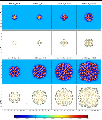
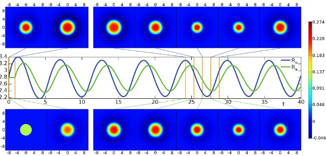
Fig. 1 Labyrinthine structure emerging from (1) and (20) with parametersβ=0.5,γ=4 and Heaviside thresholdh=0.115. The initial spot of radiusR=12 has a mode four instability, cf. Figure4. This is primed by perturbingRwith 0.5 cos(4θ ). RowsAshowuand the colorbar below indicates its values. RowsBillustrate the evolution of the interface (u=h, golden outline) due to the normal velocity of the boundary (green arrows, to scale but enlarged by a factor 50). The Liapunov functionELiap.of (2) is noted at all eight time steps. See also the video in Additional file 1.
re-placed by a lower dimensional description that evolves the boundary between high and low states of activity. This programme has already been developed by Amari in his seminal article on one-dimensional models [10], where this interface reduces nat-urally to a point (or a set of points). However, in two spatial dimensions the interface is more naturally a closed curve (or a set of closed curves).
The main topic of this article is the development of an equivalent interface de-scription for neural field models of the type exemplified by (1). We show that activity patterns can be described by dynamical equations of reduced dimension, and that these depend only on the shape of the interface (requiring no knowledge of activ-ity away from the interface). Not only is this description amenable to fast numerical simulation strategies, it allows for the construction of localized states and an anal-ysis of their linear stability. Given the computational overheads in simulating the full neural field model this enhances our ability to study pattern formation and sug-gests more generally that modeling the interfaces of patterns, rather than the patterns themselves, may lead to novel, efficient descriptions of brain activity. Indeed the use of interface dynamics to analyze patterns that arise in partial differential equation models of chemical and physical systems has a strong history [11], and it is natural to translate some of the ideas and technologies from these studies to non-local neural field models. The work by Goldstein [12,13] and Muratov [14] on pattern formation in two-dimensional excitable reaction-diffusion systems is especially relevant in this context, as both authors have developed effective descriptions of interface dynamics in terms of non-local interactions. See also the book by Desai and Kapral [15] for a recent overview.
It is worth pointing out that whether computing interface dynamics can compete with other numerical schemes will depend on the problem at hand. In general, bound-aries that remain relatively short and do not pinch guarantee a speed advantage. In practice, we expect this approach to be especially relevant for (semi-) analytical work aiming at qualitative understanding, as illustrated by some of the examples presented in this article.
localized spots occur. Moreover, we use a perturbation argument to determine the shape of traveling spots that emerge beyond a drift instability and show that spots contract in the direction of propagation and widen in the orthogonal direction. Finally, in Section7we discuss extensions of the work in this article.
2 A one-dimensional primer
Before we develop the machinery for describing the evolution of interfaces in two-dimensional neural field models, it is informative to begin with a discussion in one dimension. In this case a minimal model can be written in the form
ut= −u+ψ, ψ (x, t )=
Rw(x−y)H
u(y, t )−hdy, (3)
whereu=u(x, t ) andx ∈R, t∈R+. For a symmetric choice of synaptic kernel
w(x)=w(|x|), which decays exponentially, the one-dimensional model (3) is known to support a traveling front solution [16,17] that connects a high activity state to a low activity state. In this case it is natural to define a pattern boundary as the interface between these two states. Thus we can define a moving interface (level set) according to
ux0(t ), t
=const. (4)
Here we are assuming that there is only one point on the interface, though in principle we could consider a set of points. The functionx0=x0(t )gives the evolution of the
interface. Since the high and low activity states in the neural field model are naturally distinguished by determining whetheruis above or below the firing threshold, we shall take the constant on the right hand side of (4) to beh(though other choices are also possible). Differentiation of (4) gives an exact expression for the velocity of the interface in the form
˙
x0= −
ut
ux
x=x0(t )
. (5)
We can now describe the properties of a front solution solely in terms of the behav-ior at the front edge which separates high activity from low. To see this, let us assume that the front is such thatu(x, t ) > h for x < x0(t )andu(x, t )≤hfor x≥x0(t ).
Then (3) reduces to
ut(x, t )= −u(x, t )+
∞
x−x0(t )
w(y)dy. (6)
Introducingz=uxand differentiating (6) with respect tox gives
zt(x, t )= −z(x, t )−w
x−x0(t )
. (7)
Integrating (7) from−∞tot (and dropping transients) yields
z(x, t )= −e−t t
−∞e
swx−x
0(s)
We may now use the interface dynamics defined by (5) to study the speedc >0 of a front, defined byx˙0=c. In this casex0(t )=ct, where without loss of generality we
setx0(0)=0, and from (6) and (8) we have that
ut|x=x0(t )= −h+w(0), ux|x=x0(t )= −w(1/c)/c, (9)
where
w(λ)=
∞
0
e−λsw(s)ds. (10)
Hence from (5) the speed of the front is given implicitly by the equation
h=w(0)−w(1/c). (11) To determine stability of the traveling wave we consider a perturbation of the interface and an associated perturbation ofu. Introducing the notation· to denote perturbed quantities, to a first approximation we will setux|x=x0(t )=ux|x=ct, and
writex0(t )=ct+δx0(t ). The perturbation inu can be related to the perturbation
in the interface by noting that both the perturbed and unperturbed boundaries are defined by the level set condition, so thatu(x0, t )=h=u(x0, t ). Introducingδu(t )=
u|x=ct −u|x=x0(t ), we thus have the condition thatδu(t )=0 for allt. Integrating (6)
and dropping transients gives
u(x, t )=e−t t
−∞dse s
∞
x−x0(s)
dyw(y), (12)
anduis obtained from (12) by simply replacingx0byx0. Using the above we find
thatδuis given (to first order inδx0) by
δu(t )=1 c
∞
0
dse−s/cw(s)δx0(t )−δx0(t−s/c) =0. (13)
This has solutions of the formδx0(t )=eλt, whereλis defined byE(λ)=0, with
E(λ)=1−w(( 1+λ)/c)
w(1/c) . (14)
A front is stable if Reλ <0.
As an example consider the choicew(x)=exp(−|x|/σ )/(2σ ), for whichw(λ) = (λ+1/σ )−1/(2σ ). In this case the speed of the wave is given from (11) as
c=σ1−2h
2h , (15)
and
E(λ)= λ
1+c/σ+λ. (16)
Fig. 2 Interface parametrization and Mexican-hat shape for synaptic kernel.A: Compact areaB and boundary∂B. Two points on the boundaryr, parametrized bysands, are shown with their normalnand tangenttvectors.B: Mexican hat (20) with parametersβ=0.3 andγ=3. White contours indicate values
<0, black ones≥0, for a step size of 0.005.
Given this preliminary exposition of interface dynamics we are now ready to de-scribe the extension to two dimensions and to address the additional challenges that working in the plane gives rise to.
3 Interface dynamics in two dimensions
As in the one-dimensional case we will define pattern boundaries as the interface between low and high states of neural activity. To be more precise we introduce the notationB(t )to denote the (compact) area of activity whereu≥h. The boundary, or interface,∂B(t )is defined by the threshold crossing conditionu(x, t )=h. In this case the model defined by (1) takes the form
ut(x, t )= −u(x, t )+ψ (x, t ), ψ (x, t )=
B(t )
w|x−x|dx, (17)
and the Liapunov function can be written simply as
ELiap.[u] = − 1 2
B(t ) dx
B(t )
dxw|x−x|+h
B(t )
dx. (18)
Note thatB(t )does not have to be simply connected and can describe a union of many disjoint active regions. However, for clarity of exposition we shall focus on describing the evolution of an interface that is a single closed curve, as depicted in Figure2A. The extension to multiple closed curves is straight-forward.
can lead to azimuthal instabilities, whereby localized states can deform (or even split) into patterns with a reduced symmetry predicted by the shape of the most unstable eigenmode. Direct numerical simulations beyond such instability points have further shown the emergence of intricate spreading labyrinthine patterns like those in Fig-ure1, that leave behind a stable patterned state in their wake. It is our intention here to recover the Evans function results for stability, albeit using a purely interface de-scription of dynamics, as well as to determine the nonlinear equations of motion that govern the evolution of labyrinthine (and other) structures. Moreover, by employ-ing a representation of the synaptic connectivity in terms of a linear combination of Bessel functions, we can obtain an exact, though spatially reduced, dynamical system to describe the interface that depends solely on the shape of the interface itself. In the following, we consider kernels of the form [3]
w(r)=
N
i=1
AiK0(αir), Ai∈R, αi>0, (19)
whereK0is the zeroth order modified Bessel function of the second kind. In
partic-ular we will employ the Mexican-hat shape obtained from
w(r)= 2
3π
K0(r)−K0(2r)−
1
γ
K0(βr)−K0(2βr)
, β, γ >0, (20)
which is shown forβ=0.3 andγ=3 in Figure2B.
In an identical fashion to the way we derived an interface dynamics in one dimen-sion in Section2, we differentiateu(x, t )=halong the contour∂B(t )to obtain
∇xu·dr
dt + ∂u
∂t =0, (21)
whereris a point on the domain boundary∂Bandut and∇xuare evaluated on the boundary. Introducing the normal vector along the contour∂Basn= −∇xu/|∇xu|
allows us to obtain the normal velocity along the contour:
n·dr dt =
ut
|z|, (22)
wherez≡ ∇xu(x, t )|x=r. Using (17) we see thatuandzsatisfy
ut = −h+
Bdx
w|r−x|, (23)
zt = −z+ ∇x
Bdx
w|x−x|
x=r
. (24)
From the form of (22), (23), and (24), we see that the evolution of the interface does not require any knowledge of the neural field away from the contour, and rather just depends on the shape of the sets where the field is above threshold. We now exploit the choice ofK0as basis function for constructing the synaptic kernel to show how
elegant description of the interface dynamics that emphasizes how the geometry of
∂Bdrives the evolution of spatiotemporal patterns. The key step in this reformulation is the use of Green’s identity. For a two-dimensional vector fieldFthis identity is the two-dimensional version of the divergence theorem, which we write symbolically as
B∇ ·F=
∂BF·n. Using this first identity we may generate a second for a scalar field asB∇=∂Bn.
To evaluate the right hand side of (23) and (24) it is enough to calculate
BdxK0(α|x−x|) and its gradient. In fact, this latter term can easily be
rewrit-ten as a line integral, using the second Green’s identity, for any choice of synaptic kernel
Bdx
∇xwx−x= −
Bdx
∇xwx−x
= −
∂B
dsn(s)wx−x(s).
(25)
Using the fact thatK0(αx)satisfies the identityK0(αx)=α−2∇2K0(αx)+2π δ(αx),
as well as∇xw(|x|)=w(|x|)x/|x| andK0 = −K1, an application of Green’s first
identity shows that
Bdx
K
0
αx−x
= 1
α2
Bdx
∇2 xK0
αx−x+2π
Bdx
δαx−x (26)
= −1
α
∂B
dsn(s)· x−r(s)
|x−r(s)|K1
αx−r(s)+C2π α2.
HereC=1 ifxis withinBandC=0 ifxis outsideB. Ifxis on the boundary ofB thenC=1/2. Hence, for points on the boundary parametrized bysone finds
ut(s)= −h+ N
i=1
Ai
∂B
dsns·Ris, s+ π αi2
, (27)
zt(s)= −z(s)−
∂B
dsnswr(s)−rs, (28)
where
Ris, s= − 1 αi
r(s)−r(s)
|r(s)−r(s)|K1
αir(s)−r
s. (29)
Note that the choice ofK0as a basis forwis merely a convenience to allow explicit
calculations. As long as we can write the connectivity functionwas the divergence of a vector field then we can exploit Green’s first identity to turn the right hand side of (23) into a line integral.
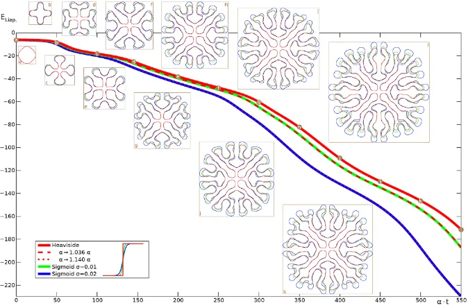
Fig. 3 Time dependence of theu=hinterface and Liapunov function.Red curvesare for the Heavi-side model of Figure1,greenandblueones use a sigmoid instead.Circular labelsindicate the times of the snapshots.Dashedanddotted curvesscale the Heaviside one by adjustingα. See also the video in Additional file 2.
reflects the expected width of the distribution of firing thresholds around a meanh
in the neural population, with the Heaviside case corresponding toσ=0. Figure3 demonstrates that for these steep sigmoids very similar labyrinthine shapes arise, and closer inspection reveals that the main differences occur at the rapidly developing rim of the structure, whereas the settled interior is nearly identical. Thus a simple adjustment of the time constantαwill in this case provide a near perfect match of the emerging structures. In Figure3we demonstrate this with the dashed and dotted red lines, which represent the Heaviside Liapunov function computed over longer time scales (up toα·t=569.9 and 626.8, respectively) and then scaled down toα·t≤550 by adjustingα. A very close match to the sigmoidal Liapunov curves (green and blue lines) is then obtained. However, for broader sigmoids we find labyrinths still re-sembling the Heaviside one, but with more obvious spatial changes. The video in Additional file 3 shows theσ=0.03 case as an example. It would seem that mild deviations in the shape of the firing rate from Heaviside (to a steep sigmoidal form) are reflected more in temporal speed than in spatial shape changes.
The Liapunov function can also be written in terms of line integrals:ELiap.= 1/2Ni=1AiFi+h, with
Fi= 1
αi2
∂B ds
∂B
dst(s)·tsK0
αir(s)−r
s−2π
αi2, (30)
where=Bdxis the area of the domain above threshold andt(s)=dr(s)/dsis the tangent vector, which can also be constructed fromnby an anti-clockwise rotation of
π/2 so that
n=
0 1
−1 0
t. (31)
To obtain (30) we have used the fact that Bdx Bdx K 0
αx−x−2π
α2
= − 1
α2
Bdx∇x·
Bdx
∇xK
0
αx−x
= − 1
α2
Bdx∇x·
∂B
dsnsK0
αx−rs
= − 1
α2 ∂B ds ∂B
dsn(s)·nsK0
αr(s)−rs,
(32)
and the observation thatn(s)·n(s)=t(s)·t(s).
ut=0 on the boundary. In this case (22) reduces to
h=
B0
dxwr−x= N
i=1
Ai
∂B0
dsns·Ris, s+ π αi2
, (33)
whereris on the boundary parametrized by s. We use the notation B0 to denote
a stationary active region. Given the stationary interface, we can also calculate the stationary fieldueverywhere (away from the interface) using (17) as
u(x)=
B0
dxwx−x, (34)
which can also be evaluated as a line integral. In order to analyze the stability of stationary solutions in the original neural field formalism defined by (1) one would perturb the field variableuand linearize to derive an eigenvalue equation or Evans function [20]. Here we determine stability using the interface dynamics, generalizing the approach described in Section2.
Using the notation·again to denote perturbed quantities, we consider small per-turbations to the contour shape and denote the new interface by∂B. The relationship between the perturbed interface and the perturbed field is, as in one dimension, de-termined by the conditionδu(t )=0, where
δu(t )=u|x∈∂B−u|x∈∂B0. (35)
The dynamics foruis given by (23) withBreplaced byB. The perturbation affects the normal vectorn(s)as well as the displacement vectorr(s)−r(s)that occurs in (27). Thus to evaluate (35) it is necessary to linearizeK1about the unperturbed
contour. In the case of interfaces without curvature the linear contribution toK1 is
zero. In contrast for curved interfaces an addition theorem for Bessel functions shows that there is a non-zero contribution. To clarify this statement and show how the above machinery is used in practice, we now give some explicit examples of localized solutions and their stability.
4 Localized states: spots
We consider spots to be circular stationary solutions. They are the equivalent of the bumps known in one spatial dimension [10]. For radially symmetric kernels we ex-pect stationary circular solutions. Yet in two spatial dimensions they can undergo azimuthalinstabilities, as already found in [6]. In order to obtain circular solutions we use the standard parametrization of a circle for the contour and write
r(θ )=R
sinθ
1−cosθ
, n(θ )=
sinθ
−cosθ
, θ∈ [0,2π ). (36)
Hence the right hand side of (33) can be calculated using
∂B
dsns·Ris, s= 1 αi
2π
0
dθK1[αiR(θ )]
R(θ ) R
2(
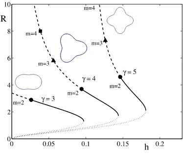
Fig. 4 Stationary radial solutions for the Mexican hat kernel (20) withβ=0.5 and various values ofγ. Thedotted branchesare circular solutions unstable to uniform changes of size.Solid branchesare stable.
Dashed branchesindicate azimuthal instabilities of different modesmwhich deform the circular solution.
whereR(θ )=R√2(1−cosθ ). Using Graf’s formula [24] to perform the integration in (37) we obtain an implicit equation for the spot radiusRin the form
h=2π
N
i=1
Ai
1
α2i − R αi
K1(αiR)I0(αiR)
, (38)
whereIν(x)is the modified Bessel function of the first kind of orderν. A plot of the spot radiusRas a function of thresholdhis shown in Figure4.
To determine the relationship between a perturbed and unperturbed spot we need to examine the conditionδu(t )=0. The general solution foru(dropping transients) can be written as
u(x, t )=e−t t
−∞dse sψ (
x, s). (39)
For a circular solution of radiusR ψis conveniently written as
ψ (r)=
2π
0
R
0
wr−rrdrdθ, r=(r, θ ). (40)
Hereψ may be constructed explicitly (off the boundary), using similar line integral calculations to those for existence (above), and is given by
ψ (r)=2π R
N
i=1
AiLi(r), (41)
where
Li(r)= ⎧ ⎪ ⎪ ⎨ ⎪ ⎪ ⎩ 1
αi
I1(αiR)K0(αir), r≥R, 1
α2iR−
1
αi
I0(αir)K1(αiR), r < R.
For perturbations in the radius of the formR=R+δR(θ, t )one finds
δu(t )=
∞
0
dse−s 2π
0
dθ
R(θ ,t−s)
0
wr−r|r=(R(θ,t ),θ ) rdr
−
R
0
wr−r|r=(R,θ )rdr
(43)
=
∞
0
dse−s 2π
0
dθδRθ−θ, t−sRwRθ+ψ(R)δR(θ, t ).
Using the above we see that δu(t )= 0 has solutions of the form δR(θ, t )=
cosmθeλmt, where
λm= −1+Wm, (44)
and
Wm=
R
|ψ(R)|
2π
0
dθcos(mθ )wR(θ )=
N
i=1AiKm(αiR)Im(αiR)
N
i=1AiK1(αiR)I1(αiR)
. (45)
Note that sinceWm is realλm∈R. A mode-minstability will occur ifλm>0, which recovers the result in [6] obtained using an Evans function approach. The pos-sibility of such azimuthal instabilities is indicated on the solution branches shown in Figure4(and we would expect the emergence of solution branches withDm symme-try from the points marked bym). Interestingly we can see from (44) and (45) that the mode withm=1 is neutrally stable. For a perturbation to a circular boundary of the formδR(θ, t )=m(t )cos(mθ ),m=eλmt and1, the perturbation of the normal velocityvnis
vn=mcos(mθ )(−1+Wm). (46)
To calculate the Liapunov function for an unperturbed spot we evaluate (30) using
1
αi2
2π
0
dθ
2π
0
dθR2cosθ−θK0
αiR
θ−θ
=4π2
αi2 R
2K
1(αiR)I1(αiR)≡Gi.
(47)
Hence
ELiap.= 1 2
N
i=1
Ai
Gi− 2π
αi2π R
2
+hπ R2. (48)
5 Rings, fronts and stripes
In this section we show how to treat other simple interface shapes, namely rings, fronts and stripes, and determine their stability. We recover previous results in [6] for rings (obtained with an Evans function method), whilst calculations for the other structures are shown to be straight-forward using the interface dynamics approach.
5.1 Rings
Rings can be considered as the difference of two spots, one with radius R1 and
the other with radiusR2> R1. Introducing ψ (r, R)=2π R
iAiLi(r, R), where
Li(r, R)is given by the right hand side of (41), we have that u(r)=ψ (r, R2)−
ψ (r, R1). Enforcing the threshold conditionsu(R2)=h=u(R1)gives a pair of
equa-tions that determine(R1, R2). To establish stability the outer contour is perturbed
exactly as in the previous section:R2(θ )=R2+aeλtcosmθ, for some small
ampli-tudea. For the inner contour we similarly writeR1(θ )=R1+beλtcosmθ. We now
generateδu(t )on each of the two boundaries and equate these to zero to generate two equations for the pair of unknown amplitudes(a, b). Demanding that this pair of equations has a non-trivial solution generates an equation forλin the formEm(λ)=0 whereEm(λ)= |(1+λ)I2−Am(λ)|and
Am(λ) μν=
Rν
|u(Rν)| 2π
0
dθcos(mθ )w
R2
μ+R2ν−2RμRνcosθ
= Rν
|u(Rν)| N
i=1
Ai
Km(αiRμ)Im(αiRν)H (Rμ−Rν) (49)
+Km(αiRν)Im(αiRμ)H (Rν−Rμ) ,
forμ, ν=1,2.
At a bifurcation point defined by Reλm=0 we expect a ring to split intomspots. In Figure5we plot solution branches for ring solutions as a function ofh for the Mexican-hat model defined by (20), and flag the types of instability that can occur. Of the two solution branches the lower one is unstable with respect to radial perturba-tions, whereas the upper branch is subject to azimuthal destabilizations. In Figure6 we show a two-dimensional plot of an unstable ring solution, and the emergent struc-ture of five bumps seen beyond instability, consistent with the predictions of our linear stability analysis.
5.2 Fronts
Calculating stationary planar fronts is straightforward, since the normal vectorn(s)
Fig. 5 Existence and stability of ring solutions with inner radiusR1, with the indicatedγ
andβ=0.5 in (20). The lower branch is always unstable (dotted lines). On theupper branchthe stable ring (solid lines) can lose stability with dominant mode=2 (solid circles), 3 (triangles), 4 (squares), etc. for decreasingh.
Fig. 6 Direct numerical simulation ofufor a ring solution (R1=7,R2=8.629) perturbed with a linear
combination of modes 0,1,2, . . . ,8. For the given parametersβ=0.5,γ=3 and Heaviside threshold
h=0.0549, modem=5 is most unstable, cf. Figure5. See also the video in Additional file 4.
To investigate the properties of a planar traveling front of speedcit is informative to treat the simple casew(x)=K0(x)/(2π ). We then have thatut= −h+1/2 and
|z| =
∞
0
dse−s
∞
−∞dy 1 2πK0
y2+(cs)2=1
2 1
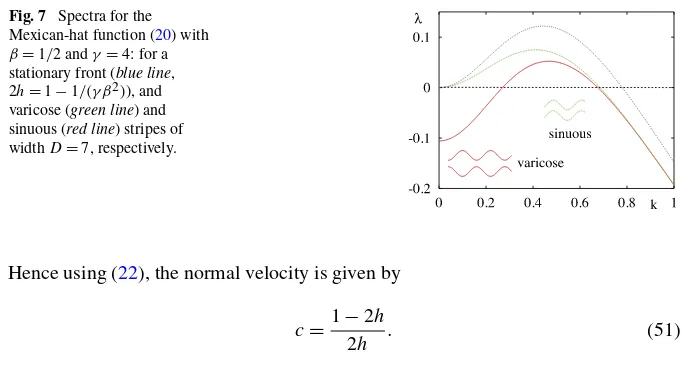
Fig. 7 Spectra for the Mexican-hat function (20) with
β=1/2 andγ=4: for a stationary front (blue line, 2h=1−1/(γ β2)), and varicose (green line) and sinuous (red line) stripes of widthD=7, respectively.
Hence using (22), the normal velocity is given by
c=1−2h
2h . (51)
To determine stability we consider a front alongy=0 and write the perturbed front asy=y(x, t ).
For simplicity we shall focus on a stationary front withc=0. In this case we may constructδu(t )as
δu(t )=
∞
0
dse−s
∞
−∞dx
y(x, t )−yx−x, t−s wx. (52)
The equationδu(t )=0 (for allx) has solutions of the formy=cos(kx)eλt, where
λ= −1+w(k)
w(0), w(k) =
∞
−∞dxw(x)cos(kx). (53) For a modified Bessel function one has
∞
−∞dxK0(αx)cos(kx)= 1
√
α2+k2. (54)
Hence for the simple example above, the stationary planar front is stable due to
w(k)≤w(0). However, for a Mexican-hat function it is possible thatw(k) >w(0)
for some band of wave numbers, and we would expect instabilities in this case. Fig-ure7showsλ=λ(k)for a stationary front with the Mexican-hat function (20), from which the critical band of wave numbers can easily be read off.
5.3 Stripes
A stripe may be considered as the active area in between two interacting stationary fronts. For two interfaces that define a stripe to be alongy=y1andy=y2, then
u(x, y)=
∞
−∞dx y2−y
y1−y
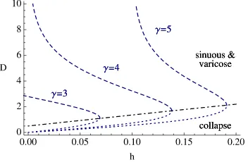
Fig. 8 Stripe widthsDfor different values ofγwith a Mexican hat interaction given by (20) andβ=0.5.
For a stripe of constant width D, such that y2−y1=D for all x, the existence
conditionu(x, y1)=h=u(x, y1+D)takes the simple form
h=
∞
−∞dx
D
0
dywx2+y2=
i
Aiπ
α2i
1−e−αiD . (56)
An example ofD=D(h)is shown in Figure8for a Mexican-hat function.
To determine stability we consider perturbations on each of the two stripe bound-aries and constructδui on each as
δui(t )=
∞
0
dse−s
∞
−∞dx
y1(x−x,t−s)−yi(x,t )
y2(x−x,t−s)−yi(x,t )
−
D
0
dywx2+y2,
(57) for i=1,2. When considering small perturbations there is some ambiguity in ex-panding (57) depending on the relative size of the perturbations on each boundary. However, this at most amounts to a sign difference, which means that we may expand (57) to obtain
δui(t )=
∞
0
dse−s
∞
−∞dx
wx2
+D2y2
x−x, t−s−yi(x, t )
±
∞
0
dse−s
∞
−∞dx
wxy
1
x−x, t−s−yi(x, t ) .
(58)
The equationsδui=0 admit solutions of the formyi =yi +icos(kx)eλt. For equal amplitude perturbations,|1| = |2| =, there are two branches of eigenvalues given byλ=λ±, where
λ±= −1+F±(k, D)
F+(0, D). (59)
HereF±(k, D)=w(k, 0)∓w(k, D) and
w(k, D)=
∞
−∞dxw
x2+D2cos(kx)=
i
Ai e−D
α2 i+k2
αi2+k2
Fig. 9 Direct numerical simulation ofufor varicose (rowsA) and sinuous (rowsB) instabilities±cos(ky)
withk=0.44272 of a stripe of widthD=6.08 for parametersβ=0.5,γ=4.0 and Heaviside threshold
h=0.03. See also the video in Additional file 5.
The branch withλ=λ+corresponds to sinuous perturbations with(1, 2)=(1,1)
and the branch withλ=λ− corresponds to varicose perturbations with (1, 2)=
(1,−1). Sinceλ+> λ−then sinuous instabilities dominate over varicose. Note that as D→ ∞ we recover the existence and stability results for a stationary front as expected. Examples of sinuous and varicose instabilities (as predicted from our anal-ysis) are shown in Figure9.
6 Neural field models with linear adaptation
In real cortical tissues there are an abundance of metabolic processes whose com-bined effect is to modulate neuronal response. It is convenient to think of these pro-cesses in terms of local feedback mechanisms that modulate synaptic currents. For example, it is known that a model of synaptic depression can destabilize a spot in favor of a traveling pulse [25]. Here we consider a simple linear model of adapta-tion that is known to lead to instabilities of localized structures [26]. In this case the original neural field model is modified according to
1
αut= −u+ψ−ga, at=u−a, (61)
may obtain the trajectory for(u, a)in closed form as
u(·, t )=
t
−∞dsη(t−s)ψ (·, s), a(·, t )= t
−∞dse
−(t−s)u(·, s), (62)
where
η(t )= α λ−−λ+
(1−λ+)e−λ+t−(1−λ−)e−λ−t. (63)
Here
λ±=1+α±
(1+α)2−4α(1+g)
2 . (64)
As an example let us compute the speed (c >0) and stability of a front in the one-dimensional model discussed in Section2 with the inclusion of a linear adaptation current. In this case we have that
ut|x=x0(t )=ch/σ, (65)
ux|x=x0(t )= −
1
c
∞
0
dsη(s/c)w(s)
= − α
c(λ−−λ+)
(1−λ+)w(λ +/c)−(1−λ−)w(λ −/c).
(66)
Note that to calculateut we have used the result thath=u(ct, t )=
∞
0 dsη(s)×
∞
cs dyw(y). Hence, from (5), the speed is determined implicitly by
h=α
2
c/σ+1
(c/σ+λ+)(c/σ+λ−), (67)
which may be rearranged to give
c σ = −
1 2
1+α− α
2h± 1+α−
α
2h
2 −4α
1+g− 1
2h
. (68)
The eigenvalue equation for stability can also be calculated, generalizing the anal-ysis of Section2, asE(λ)=1−H(λ)/H(0), where
H(λ)= α λ−−λ+
(1−λ+)w(λ+λ+)/c−(1−λ−)w(λ+λ−)/c. (69)
On the branch withc=0 where 2h(1+g)=1, defining a stationary front, we find that
E(λ)=λ(λ+λ++λ−−λ+λ−)
(λ+λ+)(λ+λ−) , (70)
In two-dimensions it is straight forward to construct a stationary spot of radiusR. This radius is determined by (38) under the replacementh→h(1+g), so that
h(1+g)=2π R
N
i=1
AiK0(αiR)I1(αiR)/αi≡F (R). (71)
Hereψmay be constructed explicitly off the boundary, and is given by Equation (41), so thatu(r)=ψ (r)/(1+g). A saddle-node bifurcation of stationary spots occurs atR=Rc whereF(Rc)=0. Hence, in the(h, g)plane stationary solutions only exist forh < F (Rc)/(1+g). Under variation in αwe expect the emergence of a drifting spot. Beyond a drift instability, we expect to be able to find traveling spots that move in some directioncwith constant speedc= |c|. These can be constructed as stationary solutions in a co-moving frameξ=x+ct, and satisfy
1
αc· ∇ξu= −u+ψ−ga, c· ∇ξa=u−a. (72)
We may write the velocity in terms of local co-ordinates on the moving interface asc=cnn+ctt, where cn(s)=c·n(s)is the normal velocity andct(s)=c·t(s) the tangential velocity at a point on the interface. Taking the cross product ofcand t(and usingn×t=1) shows that cn=c×t. Hence, the condition for stationary propagation, withc= ˙r, is
n(s)· ˙r(s)=c×dr(s) ds
! dr(s)
ds
, u(ξ )|ξ=r=h. (73)
In general this is a hard equation to solve in closed form. However, to obtain an estimate of the speed and shape of a spot beyond a point of instability it is enough to consider a weak distortion of a traveling circular wave [27]. Choosingc=c(1,0)
and writingξ=(ξ1, ξ2), and assuming thatψ is rotationally symmetric means that
we may construct a solution in the form
u(ξ1, ξ2)=
1
c
ξ1
−∞dyη
(ξ1−y)/c
ψ
y2+ξ22
. (74)
We note that the threshold conditionu=hfor a circular spot (ξ12+ξ22=R2) can only strictly be met for the casec=0, since the right hand side of (74) depends on the plane polar angle throughξ1=Rcosθ. For this case we may construct the equation
δu(t )=0 to determine the eigenvaluesλm that occur in perturbations of the form
δR(θ, t )=eλmtcos(mθ )as solutions toE
m(λ)=0, where
Em(λ)= 1
η(λ)−(1+g)Wm, (75)
whereWmis given by (44) and the Laplace transform ofηis easily calculated as
η(λ)= α(1+λ)
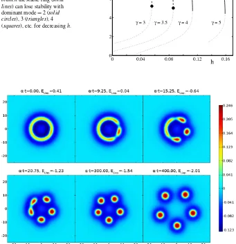
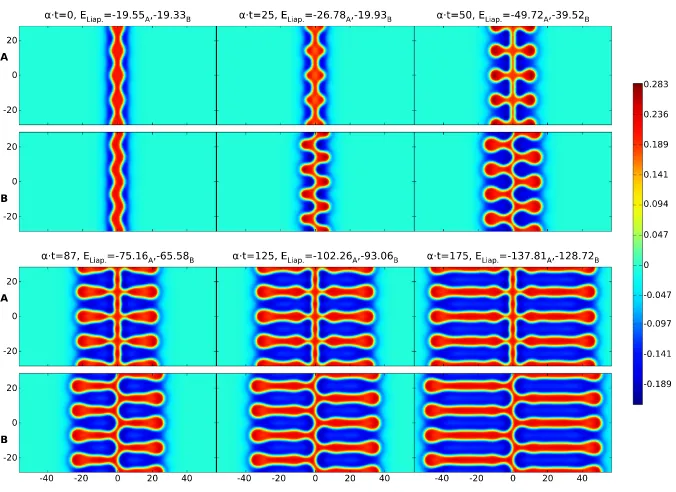
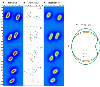
Fig. 10 Breathing instability from direct numerical simulation with parametersα=5,β=0.5,γ=4, coupling strengthg=0.5 and Heaviside thresholdh=0.12/(1+g). Initial data was constructed from a stationary spot solution by modifying the adaptation variable to a top-hat shape.Topandbottom rows: snapshots of activationuand adaptationa, respectively, at times indicated by orange lines in the middle row.Middle row: above threshold radii as function of time. See also the video in Additional file 6.
The eigenvalues form=1 are determined byη(λ)=1/(1+g), which has two solu-tions:λ=0 andλ=αg−1. Hence this mode becomes unstable asgincrease through 1/α. It is also possible that a breathing instability may arise for the mode withm=0. Note that another way to generate breathing solutions is to include localized inputs [3,4], breaking the homogeneous structure of the network. Substitution of λ=iω
into (75) gives the condition for this instability as:
W0=
1+α
α(1+g), g≥
1
α, (77)
with emergent frequencyω=√αg−1. Form≥2 splitting instabilities can be de-termined by settingλ=0 in (75) to give the conditionsWm=1. An example of a breather arising as an instability of a spot is shown in Figure10(and numerical simu-lations confirm the predicted value of the emergent frequency around the bifurcation point).
Anticipating a smallcdiscussion we Laplace transform (74) in theξ1variable to
obtain
u(λ, ξ2)=
1 1+g
1+ 1
α(1+g)
(αg−1)cλ−α(cλ)2+(cλ)3+ · · · ψ (λ, ξ2),
(78)
which we then inverse transform to obtain
u(ξ1, ξ2)=
1 1+g
1+ 1
α(1+g)
c(αg−1) ∂ ∂ξ1 −αc2 ∂
2
∂ξ12+c
3 ∂3
∂ξ13+ · · ·
ψ|ξ|.
At the point where g=1/α, the shape of the spot deviates from circular with an amplitude that depends on quadratic and higher powers ofc. Thus not only is there a breathing bifurcation atg=1/α, but also a drifting instability to a traveling spot whose shape, determined from (79) byu(r)=h, can be written in the form r(θ )=R(θ )(cosθ,sinθ )with
R(θ )=R+
m≥2
cmamcosmθ . (80)
HereRis determined by (71). A further weakly nonlinear analysis to understand the competition between drifting and breathing atg=1/αis beyond the scope of this article.
Forg >1/αand dropping terms ofO(c2)in (79) we see that there are solutions tou(r)=hof the formR(θ )=R+a1ccosθ, wherea1=(1−αg)/(α(1+g)2) <0.
The amplitudes of higher order modes may be constructed in a similar fashion, i.e., by balancing terms at each order incinu(r)=husing (79) and (80). However, it is not our intention to pursue these lengthy calculations here. Rather to give a feel of the shape of a traveling spot we plot the level set whereu(ξ1, ξ2)=husing (79)
in Figure 11D including terms up to c3. This nicely illustrates that spots contract in the direction of propagation and widen in the orthogonal direction, and provides a theoretical explanation for the shape of traveling spots recently reported in [28]. With the aid of direct numerical simulations we have also explored the scattering properties of traveling spots. In common with previous numerical studies of planar neural fields with some form of adaptation, we find that such structures can behave as quasi-particles in the sense that they can scatter like dissipative solitons [29]. An example of such scattering is shown in Figure11. Here we see a repulsive interaction which repels the spots away from each other if they approach too closely.
7 Discussion
In this article we have formulated an interface dynamics for planar neural fields with a Heaviside firing rate. This has allowed us to (i) develop an economical computa-tional framework for the evolution of spatiotemporal patterns, and (ii) perform linear stability analyses of localized structures. For simplicity we have focused on single population models. However, the extension to population models that treat the dy-namics of both excitatory and inhibitory populations is straightforward. Perhaps a more interesting extension is to consider neural field models that incorporate feature selectivity such as that observed in visual cortex for orientation [30], spatial frequency [31] and texture [32]. Denoting this feature label byχ then all of these models are expressed in terms of some non-local integro-differential equation foru(r, χ , t ). We note that the notion of an interface is still well defined and that the level set condition
Fig. 11 Collision of two pulses from direct numerical simulation with parameters as in Figure 10. ColumnsAandCshowuanda, respectively. ColumnBshows theu=hinterfaces, velocities (arrows to scale but enlarged by a factor of four), anddotted centerlinesas visual guides. See also the video in Additional file 7. ColumnDpredicts toO(c3)the shape of a traveling pulse for differentc.
Appendix: Numerical schemes
A.1 Fourier technique for neural field evolution
Because of its non-local character, the model described by (1), or its extension (61), is challenging to solve with conventional numerical methods. However, ex-ploiting the convolution structure of (1) allows one to write the Fourier transform ofR2dxw(|x−x|)f (x, t )as a product. Heref (x, t )=H (u(x, t )−h)and can be
taken either as a Heaviside or a more general sigmoidal form. Introducing a spec-tral wave-vector k then this product is simply w(|k|)f (k), where functions with argumentsk denote two-dimensional spatial Fourier transforms. We may evaluate
w(|k|)f (k)directly, at every time step, using fast Fourier transforms (FFTs). Note thatw(|k|)can be pre-computed, by FFT or here even analytically, so that the proce-dure iterated over time amounts to computingf (k)by FFT, followed by a (complex) multiplication withw(|k|), and finally an inverse FFT to obtain the result of the inte-gral. We wish to employ a parallel compute cluster for rapid computation over large grids, and hence use the free software package FFTW 3.3 [42], which includes a parallel MPI-C version. Note that the use of Fourier methods implies that the dis-cretization grid has periodic boundaries, or in other words, the solution is effectively computed on a torus. We use a grid spacing of about 0.03 or better in our computa-tions here.
In order to compute the time evolution, we use DOPRI5 [43], a well-known imple-mentation of an explicit Dormand-Prince (Runge-Kutta) method of order 5(4) with step size control and dense output of the order 4. A version in C due to J. Colinge is available on the web thanks to E. Hairer. However, in our case we perform parallel computations, so we have adapted this code accordingly using MPI-C. In particu-lar, we now consider the maximum error across all compute nodes and all variables, rather than the mean error over local variables, and communicate the resulting time step adaptation over the cluster to achieve a unified evolution of the entire distributed grid. Numerical tolerances are set to 10−7(|y
i| +1)whereyi represents all variables, i.e.,uand potentiallyaat all grid points.
This numerical method is robust against effects of the underlying grid. This is due to the employed Fourier method, which performs the spatial convolution as a multiplication in Fourier space. The discrete Fourier transform used to transfer this calculation to Fourier space calculates a trigonometric interpolation polynomial, and the influence of the grid is effectively smoothed by implicit interpolation.
Computing an evolution as shown in Additional File 1 takes several hours on the 32 to 64 Infiniband-connected compute nodes we have typically employed, and yields many gigabytes of data. We note that computation with a sigmoidal firing rate instead of the Heaviside one is over an order of magnitude faster, reflecting the numerical difficulty of dealing with sharp edges.
A.2 Interface dynamics
Equations (22) and (28) can be used to develop a numerical scheme. The contour
vectors are found by computing the orientation and distance between points. Hence the computation of the contour integrals in (28) is straight-forward and yields the normal velocity, cf. (22), which is used to displace the points of the contour in the normal direction at every time step. We employed a simple Euler method to calculate the dynamics of the contour. As the contour grows/shrinks, additional points have to be created/eliminated along the contour.
This method does not provide any means to deal with the splitting or emergence of contours. It is faster than the Fourier technique (see SectionA.1in the Appendix) for small contours, yet the time to compute the normal velocity is proportional toN2
(Nbeing the number of points discretizing the contour), as opposed toM√Mfor the Fourier technique (whereMis the number of grid points). Hence it becomes slower for larger contours due to the absence of suitable spectral methods to compute the line integrals. The main advantage of this method is the fact that no underlying grid has to be deployed across the specified domain.
Competing interests
The authors declare that they have no competing interests.
Author’s contributions
SC, HS and IB contributed equally. All authors read and approved the final manuscript.
References
1. Coombes S:Large-scale neural dynamics: simple and complex.NeuroImage2010,52:731-739. 2. Liley DTJ, Foster BL, Bojak I:Co-operative populations of neurons: mean field models of
meso-scopic brain activity. InComputational Systems Neurobiology. Edited by Le Novère, N. Berlin: Dordrecht; 2012:317-364.
3. Folias SE, Bressloff PC:Breathing pulses in an excitatory neural network.SIAM J Appl Dyn Syst
2004,3:378-407.
4. Folias SE, Bressloff PC:Breathers in two-dimensional neural media.Phys Rev Lett2005, 95(1-4):208107.
5. Kilpatrick ZP, Bressloff PC:Spatially structured oscillations in a two-dimensional excitatory neu-ronal network with synaptic depression.J Comput Neurosci2010,28:193-209.
6. Owen MR, Laing CR, Coombes S:Bumps and rings in a two-dimensional neural field: splitting and rotational instabilities.New J Phys2007,9:378.
7. French DA:Identification of a free energy functional in an integro-differential equation model for neuronal network activity.Appl Math Lett2004,17:1047-1051.
8. Kenet T, Bibitchkov D, Tsodyks M, Grinvald A, Arieli A:Spontaneously emerging cortical repre-sentations of visual attributes.Nature2003,425:954-956.
9. Sadaghiani S, Hesselmann G, Friston KJ, Kleinschmidt A:The relation of ongoing brain activity, evoked neural responses, and cognition.Front Syst Neurosci2010,4:20.
10. Amari S:Dynamics of pattern formation in lateral-inhibition type neural fields.Biol Cybern
1977,27:77-87.
11. Pismen LM:Patterns and Interfaces in Dissipative Dynamics. Berlin: Springer; 2006. [Springer Series in Synergetics.]
13. Goldstein RE:Nonlinear dynamics of pattern formation in physics and biology. InPattern For-mation in the Physical and Biological Sciences. Reading: Addison-Wesley; 1997:65-91.
14. Muratov CB:Theory of domain patterns in systems with long-range interactions of Coulomb type.Phys Rev E2002,66(1-25):066108.
15. Desai RC, Kapral R:Dynamics of Self-Organized and Self-Assembled Structures. Cambridge: Cam-bridge University Press; 2009.
16. Ermentrout GB, McLeod JB:Existence and uniqueness of travelling waves for a neural network.
Proc R Soc Edinb, Sect A, Math1993,123:461-478.
17. Coombes S:Waves, bumps and patterns in neural field theories.Biol Cybern2005,93:91-108. 18. Taylor JG:Neural ‘bubble’ dynamics in two dimensions: foundations.Biol Cybern1999,
80:393-409.
19. Werner H, Richter T:Circular stationary solutions in two-dimensional neural fields.Biol Cybern
2001,85:211-217.
20. Coombes S, Owen MR:Evans functions for integral neural field equations with Heaviside firing rate function.SIAM J Appl Dyn Syst2004,34:574-600.
21. Laing CR, Troy WC:PDE methods for nonlocal models.SIAM J Appl Dyn Syst2003,2:487-516. 22. Pullin DI:Contour dynamics methods.Annu Rev Fluid Mech1992,24:89-115.
23. Zabusky NJ, Hughes MH, Roberts KV:Contour dynamics for the Euler equations in two dimen-sions.J Comput Phys1997,135:220-226.
24. Watson GN:A Treatise on the Theory of Bessel Functions. Cambridge: Cambridge University Press; 2006.
25. Bressloff PC, Kilpatrick ZP:Two-dimensional bumps in piecewise smooth neural fields with synaptic depression.SIAM J Appl Math2011,71:379-408.
26. Pinto DJ, Ermentrout GB:Spatially structured activity in synaptically coupled neuronal net-works: I. Travelling fronts and pulses.SIAM J Appl Math2001,62:206-225.
27. Pismen LM:Nonlocal boundary dynamics of traveling spots in a reaction-diffusion system.Phys Rev Lett2001,86:548-551.
28. Lu Y, Amari S:Traveling bumps and their collisions in a two-dimensional neural field.Neural Comput2011,23:1248-1260.
29. Coombes S, Owen MR:Exotic dynamics in a firing rate model of neural tissue with threshold accommodation. InFluids and Waves: Recent Trends in Applied Analysis. Providence: Am. Math. Soc.; 2007:123-144. [Contemp. Math., vol 440.]
30. Ben-Yishai R, Bar-Or L, Sompolinsky H:Theory of orientation tuning in visual cortex.Proc Natl Acad Sci USA1995,92:3844-3848.
31. Bressloff PC, Cowan JD:Spherical model of orientation and spatial frequency tuning in a cortical hypercolumn.Philos Trans R Soc Lond B2003,358:1643-1667.
32. Faye G, Chossat P, Faugeras O:Analysis of a hyperbolic geometric model for visual texture per-ception.J Math Neurosci2011,1:4.
33. Petitot J:The neurogeometry of pinwheels as a sub-Riemannian contact structure.J Physiol
2003,97:265-309.
34. Coombes S, Schmidt H:Neural fields with sigmoidal firing rates: approximate solutions.Discrete Contin Dyn Syst, Ser A2010,28:1369-1379.
35. Coombes S, Owen MR:Bumps, breathers, and waves in a neural network with spike frequency adaptation.Phys Rev Lett2005,94:148102.
36. Bojak I, Liley DTJ:Axonal velocity distributions in neural field equations.PLoS Comput Biol
2010,6:e1000653.
37. Hagberg A, Meron E:Order parameter equations for front transitions: nonuniformly curved fronts.Physica D1998,123:460-473.
38. Kawaguchi S, Mimura M:Collision of travelling waves in a reaction-diffusion system with global coupling effect.SIAM J Appl Math1999,59:920-941.
39. Ohta T:Pulse dynamics in a reaction-diffusion system.Physica D2001,151:61-72.
40. Bressloff PC:Weakly-interacting pulses in synaptically coupled neural media.SIAM J Appl Math
2005,66:57-81.
41. Venkov NA:Dynamics of neural field models.PhD thesis. School of Mathematical Sciences, Uni-versity of Nottingham; 2009. [http://www.umnaglava.org/pdfs.html]
42. Frigo M, Johnson SG:The design and implementation of FFTW3.Proc IEEE2005, 93(2):216-231.