Subdivision Matrices and Iterated Function Systems for Parametric Interval Bezier Curves

(1)

170602-9494-IJVIPNS-IJENS © April 2017 IJENS

Subdivision Matrices and Iterated Function

Systems for Parametric Interval Bezier Curves

O. Ismail, Senior Member, IEEE

Abstract— Fractals are famous both for their strange appearance and for their odd geometric properties. The problem of modeling is very simple when one has mathematical description of the fractal he wants to model. A set of transformations that generates a fractal by iteration is called an iterated function systems (IFS). An iterated function system maps the corresponding fractal onto itself as a collection of smaller self-similar copies. Fractals are often defined as fixed points of iterated function systems because when applied to the fractal the transformations that generate a fractal do not alter the fractal. In this paper we are going to show that the parametric interval Bezier curves are indeed fractals if the four fixed Kharitonov's polynomials (four fixed Bezier curves) associated with the original interval Bezier curves are fractals. The four fixed Kharitonov's polynomials (four fixed Bezier curves) associated with the original parametric interval Bezier curve are obtained. Iterated function systems (IFS) for the four fixed Kharitonov's polynomials (four fixed Bezier curves) are constructed so that starting with any compact set, not just the four fixed Kharitonov's polynomials (four fixed Bezier curves) control polygons, and iterating the transformations, the resulting sets converge in the limit to the given four fixed Kharitonov's polynomials (four fixed Bezier curves) curves. The transformation matrices in the iterated function systems are constructed to mimic the subdivision procedure, so there is indeed a deep connection between subdivision algorithms and fractal procedures. The fixed control points that subdivide the four fixed Kharitonov's polynomials (four fixed Bezier curves) curves into two four fixed Kharitonov's polynomials (four fixed Bezier curves) curves are affine combinations of the original four fixed Kharitonov's polynomials (four fixed Bezier curves) control points. Thus we can represent the four fixed Kharitonov's polynomials (four fixed Bezier curves) subdivision by two square matrices whose entries are the coefficients in these affine combinations. A numerical example is included in order to demonstrate the effectiveness of the proposed method.

Index Terms— Subdivision matrices, iterated function systems, interval Bezier curve, CAGD.

I. INTRODUCTION

Parametric representations are widely used since they allow considerable flexibility for shaping and design. In computer aided design and geometric modeling, there are considerable interests in approximating curves and surfaces with simpler forms of curves and surfaces. Parametric Bezier curves are interactive. It is possible to control the shape of the Bezier curve by moving the control points and by smoothly connecting individual segments.

The Bezier curve possesses a characteristic intuitiveness in expressing the desired shape through property of convexity of control polygon. Interestingly during the same time, de Casteljau too adopted Bernstein Basis for his work which was

The author is with Department of Computer Engineering, Faculty of Electrical and Electronic Engineering, University of Aleppo, Aleppo, (e-mail:[email protected]).

focused on the property of non-negativity and partition of unity of the basis function associated with the control points. Subdivision of the Bezier curve is required to break the curve into number of small segments for various applications like curve fitting, segmentation, interpolation, and so. Besides some key Bernstein basis properties that constraints the behavior of Bezier curve like symmetry, recursion, non-negativity, unity of partition, unimodality, relation to monomial basis, lower and upper bounds, variation diminishing property, derivatives and integrals there are some algorithms based properties like degree elevation, degree reduction and composition that have consistently been evaluated and analyzed over a period of decades in order to broaden its applications.

There are several kinds of polynomial curves in CAGD, e.g., Bezier [1], [2], [3], [4] Said-Ball [5], Wang-Ball [6], [7], [8], B-spline curves [9] and DP curves [10], [11]. These curves have some common and different properties. All of them are defined in terms of the sum of product of their blending functions and control points. They are just different in their own basis polynomials. In order to compare these curves, we need to consider these properties. The common properties of these curves are control points, weights, and their number of degrees. Control points are the points that affect to the shape of the curve. Weights can be treated as the indicators to control how much each control point influences to the curve. Number of degree determines the maximum degree of polynomials. In different curves, these properties are not computed by the same method. To compare different kinds of curves we need to convert these curves into an intermediate form.

A parametric interval Bezier curve [12-18] is a Bezier curve whose control points are rectangles (the sides of which are parallel to coordinate axis) in a plane.

The control points that subdivide a Bezier curve into two Bezier curves are affine combinations of the original Bezier control points. Thus we can represent Bezier subdivision by two square matrices whose entries are the coefficients in these affine combinations.

(2)

170602-9494-IJVIPNS-IJENS © April 2017 IJENS used in image coding. Fractals are attractors-fixed points of

iterated function systems (𝐼𝐹𝑆) [19], [20], [21]. The fractal methods became very important tools in many disciplines and found very wide practical applications e.g., image compression, generating shore lines, mountains, clouds, pattern recognition, image processing, computer graphics or in medicine and economy. In computer graphics, there is a need for succinct description of a complex object’s geometry and an efficient way to vary the geometry of an object to make movies.

In this paper it has been shown that if the four fixed Kharitonov's polynomials (four fixed Bezier curves) associated with the original parametric interval Bezier curve are fractals; then the given parametric interval Bezier curve is fractal.

This paper is organized as follows. Section II contains the basic results, whereas section III shows a numerical example, and the final section offers conclusions.

II.THEBASICRESULTS

Parametric interval Bezier curves are segments of parametric interval polynomial curves. Each piece of a parametric interval polynomial curve is just like any other piece of a parametric interval polynomial curve, so each segment of a parametric interval Bezier curve is itself a parametric interval Bezier curve. Thus, parametric interval Bezier curves are self-similar. Therefore, even though the parametric interval Bezier curves are infinitely differentiable, the interval Bezier curves are also fractal interval curves.

Let {[𝑝_𝑖−_{, 𝑝}

𝑖+]}𝑖=0𝑛 be a given set of interval control points which defines the interval Bezier curve:

𝑃𝑛𝐼(𝑢) = ∑[𝑝𝑖−, 𝑝𝑖+] 𝑛

𝑖=0

𝐵𝑖𝑛(𝑢)

= ∑([𝑥𝑖−, 𝑥𝑖+], [𝑦𝑖−, 𝑦𝑖+]) 𝑛

𝑖=0

𝐵𝑖𝑛(𝑢)

0 ≤ 𝑢 ≤ 1

(1) of degree 𝑛 where {𝐵_𝑘𝑛(𝑢)}_𝑘=0𝑛 are Bernstein polynomials formed by:

𝐵_𝑘𝑗(𝑢) = (𝑗

𝑘) (1 − 𝑢)(𝑗−𝑘)𝑢𝑘 , (𝑘 = 0, 1, ⋯ , 𝑗) (2)

and

(𝑗 𝑘) =

𝑗! 𝑘! (𝑗 − 𝑘)!

is a binomial coefficient.

The sufficient condition for the given parametric interval Bezier curves to be fractals is that the four fixed Kharitonov's polynomials (four fixed Bezier curves) associated with the parametric interval Bezier curve should be fractals. Now the interval Bezier curve 𝑃𝑛𝐼(𝑢) for 𝑢 ∈ [0,1] is fractal, if the four fixed Kharitonov's polynomials (four fixed Bezier curves) 𝑃𝑛𝑗(𝑢) for 𝑢 ∈ [0,1] and 𝑗 = 1,2,3,4 are fractals. The four

fixed Kharitonov's polynomials (four fixed Bezier curves) [22] associated with the original parametric interval Bezier curve are:

𝑃𝑛1(𝑢) = 𝑝0−𝐵0𝑛(𝑢) + 𝑝1−𝐵1𝑛(𝑢) + 𝑝2+𝐵2𝑛(𝑢) + 𝑝3+𝐵3𝑛(𝑢) + 𝑝4−𝐵4𝑛(𝑢) + 𝑝5−𝐵5𝑛(𝑢) + ⋯

≡ 𝛼0,𝑛1 𝐵0𝑛(𝑢) + 𝛼1,𝑛1 𝐵1𝑛(𝑢) + 𝛼2,𝑛1 𝐵2𝑛(𝑢) + ⋯ + 𝛼𝑛,𝑛1 𝐵𝑛𝑛(𝑢)

𝑃𝑛2(𝑢) = 𝑝0−𝐵0𝑛(𝑢) + 𝑝1+𝐵1𝑛(𝑢) + 𝑝2+𝐵2𝑛(𝑢) + 𝑝3−𝐵3𝑛(𝑢) + 𝑝4−𝐵4𝑛(𝑢) + 𝑝5+𝐵5𝑛(𝑢) + ⋯

𝑃𝑛3(𝑢) = 𝑝0+𝐵0𝑛(𝑢) + 𝑝1+𝐵1𝑛(𝑢) + 𝑝2−𝐵2𝑛(𝑢) + 𝑝3−𝐵3𝑛(𝑢) + 𝑝4+𝐵4𝑛(𝑢) + 𝑝5+𝐵5𝑛(𝑢) + ⋯

𝑃𝑛4(𝑢) = 𝑝0+𝐵0𝑛(𝑢) + 𝑝1−𝐵1𝑛(𝑢) + 𝑝2−𝐵2𝑛(𝑢) + 𝑝3+𝐵3𝑛(𝑢) + 𝑝4+𝐵4𝑛(𝑢) + 𝑝5−𝐵5𝑛(𝑢) + ⋯

≡ 𝛼0,𝑛4 𝐵0𝑛(𝑢) + 𝛼1,𝑛4 𝐵1𝑛(𝑢) + 𝛼2,𝑛4 𝐵2𝑛(𝑢) + ⋯ + 𝛼𝑛,𝑛4 𝐵𝑛𝑛(𝑢) (3) The four fixed Kharitonov's polynomials (four fixed Bezier curves) can be written as follows:

𝑃𝑛𝑗(𝑢) = ∑ 𝛼𝑖,𝑛𝑗 𝑛

𝑖=0

𝐵𝑖𝑛(𝑢)

₍₄₎𝑓𝑜𝑟 𝑎𝑙𝑙 𝑢 ∈ [0,1] 𝑎𝑛𝑑 (𝑗 = 1,2,3,4)

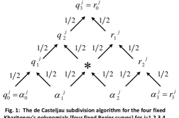
The de Casteljau evaluation algorithm for the four fixed Kharitonov's polynomials (four fixed Bezier curves) is also a subdivision procedure, if we run the de Casteljau evaluation algorithm at the midpoint of the parameter interval [𝑎, 𝑏], then the fixed control points of the four fixed Kharitonov's polynomials (four fixed Bezier curves) that subdivide the four fixed Kharitonov's polynomials (four fixed Bezier curves) at 𝑢 = (𝑎 + 𝑏) 2⁄ emerge along the left and right lateral edges of the de Casteljau triangle as shown below in Figure 1 . Moreover, the labels along each edge in this triangle are 1 2⁄ , independent of the choice of the parameter interval. Our initial goal is to develop explicit expressions for the fixed control points 𝑞0𝑗, 𝑞1𝑗, ⋯ , 𝑞𝑛𝑗 and 𝑟0𝑗, 𝑟1𝑗, ⋯ , 𝑟𝑛𝑗 of the four fixed Kharitonov's polynomials (four fixed Bezier curves) that subdivide the four fixed Kharitonov's polynomials (four fixed Bezier curves) of degree 𝑛 in terms of the original control points 𝛼₀𝑗, 𝛼₁𝑗, ⋯ , 𝛼_𝑛𝑗 of the four fixed Kharitonov's polynomials (four fixed Bezier curves). Such formulas are easy to ﬁnd.

j j q00

2

1 12

j q1

2 1 2 1

j q2

j j

r q3 0

2 1

2

1



2 1

j r1

j r2

2 1

j j

r3 3 

j 2 

j 1 

Fig. 1: The de Casteljau subdivision algorithm for the four fixed Kharitonov's polynomials (four fixed Bezier curves) for j=1,2,3,4.

2

1 12

(3)

170602-9494-IJVIPNS-IJENS © April 2017 IJENS {

𝑞_𝑙𝑗₌ 1

2𝑙∑ 𝑝(𝑙, 𝑚)𝛼𝑚𝑗 𝑙

𝑚=0

𝑟_𝑛−𝑙𝑗 = 1

2𝑙 ∑ 𝑝(𝑙, 𝑚)𝛼𝑛−𝑚𝑗 𝑙

𝑚=0 }

(𝑗 = 1,2,3,4)

(5)

where 𝑝(𝑙, 𝑚) is the number of paths from 𝛼_𝑚𝑗 to 𝑞_𝑙𝑗 or equivalently from 𝛼𝑛−𝑚𝑗 to 𝑟𝑛−𝑙𝑗 . But the number of paths from the 𝑚𝑡ℎ_{position at the base to the apex of a triangle is} the same as the number of paths from the apex to the 𝑚𝑡ℎ position at the base of a triangle. The number of paths from the apex to any node in a triangle is given by the values in the nodes of Pascal’s triangle that is, by binomial coefﬁcients.

Therefore, 𝑝(𝑙, 𝑚) = ( 𝑙_𝑚), so

{ 𝑞_𝑙𝑗₌ 1

2𝑙∑ ( 𝑙_𝑚) 𝛼𝑚𝑗 𝑙

𝑚=0

, 𝑙 = 0,1, ⋯ , 𝑛

𝑟_𝑛−𝑙𝑗 = 1

2𝑙∑ ( 𝑙_𝑚) 𝛼𝑛−𝑚𝑗 𝑙

𝑚=0

, 𝑙 = 0,1, ⋯ , 𝑛 }

(𝑗 = 1,2,3,4)

(6)

Using Equation (6), we can represent the fixed points 𝑞0𝑗, 𝑞1𝑗, ⋯ , 𝑞𝑛𝑗 and 𝑟0𝑗, 𝑟1𝑗, ⋯ , 𝑟𝑛𝑗 that subdivide the four fixed Kharitonov's polynomials (four fixed Bezier curves) using matrix multiplication. Let 𝐻(𝑛) be the (2𝑛 + 1) × (𝑛 + 1) matrix deﬁned by:

𝐻(𝑛) =

[

1 0 ⋯ ⋯ 0

1 2

1

2 ⋯ ⋯ 0

⋮ ⋮ ⋮ ⋮

1 2𝑛

𝑛 2𝑛 ⋯ ⋯

1 2𝑛

0 1

2𝑛 ⋯ ⋯ 1 2𝑛

⋮ ⋮ ⋯ ⋯ ⋮

0 0 ⋯ ⋯ 1 ]

(𝑗 = 1,2,3,4)

(7)

Then, using equation (6), we can write:

𝐻(𝑛) ∙

[ 𝛼0𝑗

𝛼₁𝑗 ⋮ ⋮ 𝛼𝑛𝑗]

=

[ 𝑞0𝑗

𝑞₁𝑗 ⋮ ⋮ 𝑞𝑛𝑗 = 𝑟0𝑗

𝑟₁𝑗 ⋮ ⋮ 𝑟𝑛𝑗 ]

(𝑗 = 1,2,3,4)

(8)

We can split 𝐻(𝑛) into two square (𝑛 + 1) × (𝑛 + 1) matrices 𝐿(𝑛) and 𝑅(𝑛), where 𝐿(𝑛) consists of the ﬁrst (𝑛 + 1) rows and 𝑅(𝑛) the last (𝑛 + 1) rows of 𝐻(𝑛). Thus,

𝐿(𝑛) =

[

1 0 ⋯ ⋯ 0

1 2

1

2 ⋯ ⋯ 0

⋮ ⋮ ⋯ ⋯ ⋮

1 2𝑛

𝑛 2𝑛 ⋯ ⋯

1 2𝑛]

=( 𝑙𝑚) 2𝑙

(𝑙, 𝑚 = 0,1, ⋯ , 𝑛) (𝑗 = 1,2,3,4)

(9)

and

𝑅(𝑛) =

[ 1 2𝑛

𝑛

2𝑛 ⋯ ⋯

1 2𝑛

0 1

2𝑛−1 ⋯ ⋯ 1 2𝑛−1

⋮ ⋮ ⋯ ⋯ ⋮

0 0 ⋯ ⋯ 1 ]

=( 𝑛 − 𝑙𝑛 − 𝑚) 2𝑛−𝑙

(𝑙, 𝑚 = 0,1, ⋯ , 𝑛) (𝑗 = 1,2,3,4)

(10)

where, the matrices 𝐿(𝑛) and 𝑅(𝑛), represent left and right subdivision for the four fixed Kharitonov's polynomials (four fixed Bezier curves).

Therefore, we can write:

𝐿(𝑛) ∙

[ 𝛼0𝑗

𝛼1𝑗 ⋮ ⋮ 𝛼𝑛𝑗]

=

[

1 0 ⋯ ⋯ 0

1 2

1

2 ⋯ ⋯ 0

⋮ ⋮ ⋯ ⋯ ⋮

1 2𝑛

𝑛 2𝑛 ⋯ ⋯

1 2𝑛_]

∙

[ 𝛼0𝑗

=

[ 𝑞0𝑗

𝑞1𝑗 ⋮ ⋮ 𝑞𝑛𝑗]

(𝑗 = 1,2,3,4)

(11)

and

𝑅(𝑛) ∙

[ 𝛼0𝑗

=

[ 1 2𝑛

𝑛

2𝑛 ⋯ ⋯

1 2𝑛

0 1

2𝑛−1 ⋯ ⋯ 1 2𝑛−1

⋮ ⋮ ⋯ ⋯ ⋮

0 0 ⋯ ⋯ 1 ]

∙

[ 𝛼0𝑗

=

[ 𝑟0𝑗

𝑟1𝑗 ⋮ ⋮ 𝑟𝑛𝑗]

(𝑗 = 1,2,3,4)

(12)

(4)

170602-9494-IJVIPNS-IJENS © April 2017 IJENS row of 𝐿(𝑛) is the same as the ﬁrst row of 𝑅(𝑛) because 𝑞𝑛𝑗 =

𝑟𝑛𝑗.

Starting with the original four fixed Kharitonov's polynomials (four fixed Bezier curves) control points and applying these matrices repeatedly generates a sequence of fixed control polygons that converge to the original four fixed Kharitonov's polynomials (four fixed Bezier curves) [23], [24].

Suppose, however, that the matrices 𝛼𝑗= [𝛼0𝑗 𝛼1𝑗 ⋯ ⋯ 𝛼𝑛𝑗]

𝑇

are invertible. Let

{

𝐿𝑝𝑗(𝑛) = [𝛼𝑗]−1∙ 𝐿(𝑛) ∙ 𝛼𝑗 𝑅𝑝𝑗(𝑛) = [𝛼𝑗]−1∙ 𝑅(𝑛) ∙ 𝛼𝑗 (𝑗 = 1,2,3,4)

} (13)

Then,

{ 𝛼𝑗_{∙ 𝐿}

𝑝

𝑗_{(𝑛) = 𝛼}𝑗_{∙ ([𝛼}𝑗_]−1_{∙ 𝐿(𝑛) ∙ 𝛼}𝑗_{) = 𝐿(𝑛) ∙ 𝛼}𝑗

𝛼𝑗_{∙ 𝑅}

𝑝𝑗(𝑛) = 𝛼𝑗∙ ([𝛼𝑗]−1∙ 𝑅(𝑛) ∙ 𝛼𝑗) = 𝑅(𝑛) ∙ 𝛼𝑗 (𝑗 = 1,2,3,4)

}

(14) Moreover, iterating the transformations 𝐿𝑗𝑝(𝑛) and 𝑅𝑝𝑗(𝑛) multiplying now on the right instead of on the left generates the same sequence of four fixed Kharitonov's polynomials (four fixed Bezier curves) control polygons as iterating the matrices 𝐿(𝑛) and 𝑅(𝑛) on the control polygons 𝛼𝑗_{for (𝑗 = 1,2,3,4). But, and this is the key point, it is easy} to show that the matrices 𝐿_𝑝𝑗(𝑛) and 𝑅_𝑝𝑗(𝑛), represent contractive maps. Therefore {𝐿_𝑝𝑗(𝑛), 𝑅_𝑝𝑗(𝑛)} for (𝑗 = 1,2,3,4) are iterated function systems, so we can start with any compact set and the iteration will still converge to the four fixed Kharitonov's polynomials (four fixed Bezier curves) with fixed control points 𝛼₀𝑗, 𝛼₁𝑗, ⋯ , 𝛼𝑛𝑗 for (𝑗 = 1,2,3,4).

For the four fixed Kharitonov's polynomials (four fixed Bezier curves) of degree 𝑛 , the subdivision matrices 𝐿(𝑛) and 𝑅(𝑛), are (𝑛 + 1) × (𝑛 + 1) matrices. To form the matrices 𝐿𝑗_𝑝(𝑛) and 𝑅_𝑝𝑗(𝑛) for (𝑗 = 1,2,3,4) the coordinates of the four fixed Kharitonov's polynomials (four fixed Bezier curves) control points 𝛼𝑗= [𝛼₀𝑗 𝛼₁𝑗 ⋯ ⋯ 𝛼_𝑛𝑗]𝑇 must constitute invertible (𝑛 + 1) × (𝑛 + 1) matrices. If the fixed points 𝛼₀𝑗, 𝛼₁𝑗, ⋯ , 𝛼_𝑛𝑗 lie in an 𝑛 − 𝑑𝑖𝑚𝑒𝑛𝑠𝑖𝑜𝑛𝑎𝑙 affine space, then we can use homogeneous coordinates to form (𝑛 + 1) × (𝑛 + 1) matrices.

𝛼𝑗_{= [𝛼}₀𝑗 𝛼₁𝑗 ⋯ ⋯ 𝛼𝑛𝑗

1 1 ⋯ ⋯ 1]

𝑇

(𝑗 = 1,2,3,4)

(15) The matrices 𝛼𝑗 for (𝑗 = 1,2,3,4) are then invertible precisely when the fixed points 𝛼₀𝑗, 𝛼₁𝑗, ⋯ , 𝛼𝑛𝑗 are affinely independent. Typically, however, the degree n of the four fixed Kharitonov's polynomials (four fixed Bezier curves) is larger than the dimension 𝑑 of the ambient space of the fixed control points. For example, for planar cubic curves,

𝑛 = 3 but 𝑑 = 2 . Nevertheless, in general, we can still form the matrices 𝐿𝑗𝑝(𝑛) and 𝑅𝑝𝑗(𝑛), by lifting the fixed control points 𝛼𝑗= [𝛼₀𝑗 𝛼₁𝑗 ⋯ ⋯ 𝛼_𝑛𝑗]𝑇 to higher dimensions.

For planar four fixed Kharitonov's polynomials (four fixed Bezier curves), we can proceed in the following fashion. Let (𝑥_𝑘𝑗, 𝑦_𝑘𝑗) for (𝑗 = 1,2,3,4) be the rectangular coordinates of 𝛼_𝑘𝑗, for 𝑘 = 0,1, ⋯ , 𝑛. Then we can lift 𝛼𝑗to higher dimensions by introducing homogeneous coordinates and lifting each four fixed Kharitonov's polynomials (four fixed Bezier curves) control point 𝛼_𝑘𝑗to dimension 𝑘, 3 ≤

𝑘 ≤ 𝑛, by annexing zeroes and ones to the coordinates of 𝛼_𝑘𝑗

for (𝑗 = 1,2,3,4) and 𝑘 = 0,1, ⋯ , 𝑛. For example, for cubics we introduce one additional coordinate and set:

𝛼𝑗₌

[

𝛼0𝑗 1 0 𝛼₁𝑗 1 0 𝛼2𝑗 1 0 𝛼3𝑗 1 1]

=

[

𝑥0𝑗 𝑦0𝑗 1 0 𝑥₁𝑗 𝑦₁𝑗 1 0 𝑥2𝑗 𝑦2𝑗 1 0 𝑥3𝑗 𝑦3𝑗 1 1] (𝑗 = 1,2,3,4)

(16)

and for quartics we introduce two additional coordinates and set:

𝛼𝑗₌

[

𝛼0𝑗 1 0 0 𝛼1𝑗 1 0 0 𝛼2𝑗 1 0 0 𝛼3𝑗 1 1 0 𝛼4𝑗 1 1 1]

=

[

𝑥0𝑗 𝑦0𝑗 1 0 0 𝑥1𝑗 𝑦1𝑗 1 0 0 𝑥2𝑗 𝑦2𝑗 1 0 0 𝑥3𝑗 𝑦3𝑗 1 1 0 𝑥4𝑗 𝑦4𝑗 1 1 1] (𝑗 = 1,2,3,4)

(17)

and so on. We notice that in each case, the matrix 𝛼𝑗 is invertible if:

𝑑𝑒𝑡 [ 𝛼₀𝑗 1 𝛼₁𝑗 1 𝛼₂𝑗 1

] ≠ 0

(𝑗 = 1,2,3,4)

(18) Thus, 𝛼𝑗_{is invertible if the points 𝛼}

0𝑗, 𝛼1𝑗 , 𝛼2𝑗, are affinely independent; that is, if the points 𝛼0𝑗, 𝛼1𝑗 , 𝛼2𝑗, are not collinear. Of course, we could choose any other three non collinear fixed control points and this lifting technique would work equally well.

(5)

Kharitonov's polynomials (four fixed Bezier curves) orthogonally back down to the original dimension 𝑑.

III.NUMERICALEXAMPLE

Consider the case of quadratic parametric interval Bezier curve 𝑃2𝐼(𝑢) for 0 ≤ 𝑢 ≤ 1.

𝑃2𝐼(𝑢) = ∑[𝑝𝑖−, 𝑝𝑖+] 2

𝑖=0

𝐵𝑖2(𝑢)

= ∑([𝑥𝑖−, 𝑥𝑖+], [𝑦𝑖−, 𝑦𝑖+]) 2

𝑖=0

𝐵𝑖2(𝑢)

0 ≤ 𝑢 ≤ 1

Here, 𝑛 = 2, so the subdivision matrices 𝐿(2) and 𝑅(2) are 3 × 3 matrices, which at least are the right size matrices for generating fractals in the plane. As explained in section II the matrices 𝐿(2) and 𝑅(2) are obtained as follows:

𝐿(2) =

[

1 0 0 1 2

1

2 0

1 4

2 4

1 4]

, 𝑅(2) =

[ 1 4

2 4

1 4

0 1

2 1 2 0 0 1]

Unfortunately, it is not clear what happens to an arbitrary point when we multiply by these matrices on the right. But suppose that instead of the matrices 𝐿(2) and 𝑅(2), we let:

𝛼𝑗_{= [} 𝛼₀𝑗 1 𝛼₁𝑗 1 𝛼₂𝑗 1

] = [

𝑥₀𝑗 𝑦₀𝑗 1 𝑥₁𝑗 𝑦₁𝑗 1 𝑥₂𝑗 𝑦₂𝑗 1 ]

(𝑗 = 1,2,3,4)

be the matrices of the four fixed Kharitonov's polynomials (four fixed Bezier curves) control points and we consider the matrices:

{

𝐿𝑝𝑗(2) = [𝛼𝑗]−1∙ 𝐿𝑗(2) ∙ 𝛼𝑗 𝑅𝑝𝑗(2) = [𝛼𝑗]−1∙ 𝑅𝑗(2) ∙ 𝛼𝑗 (𝑗 = 1,2,3,4)

}

Applying these matrices to the four fixed Kharitonov's polynomials (four fixed Bezier curves) control points 𝛼𝑗_on the right yields:

{ 𝛼𝑗_{∙ 𝐿}

𝑝

𝑗_{(2) = 𝛼}𝑗_{∙ ([𝛼}𝑗_]−1_{∙ 𝐿(2) ∙ 𝛼}𝑗_{) = 𝐿(2) ∙ 𝛼}𝑗

𝛼𝑗_{∙ 𝑅}

𝑝𝑗(2) = 𝛼𝑗∙ ([𝛼𝑗]−1∙ 𝐿(2) ∙ 𝛼𝑗) = 𝑅(2) ∙ 𝛼𝑗 (𝑗 = 1,2,3,4)

}

Furthermore, if we iterate this procedure by continuing to apply the matrices 𝐿𝑗𝑝(2) and 𝑅𝑝𝑗(2) on the right, then we get exactly the same points that are generated by applying the matrices 𝐿(2) and 𝑅(2) to the four fixed Kharitonov's polynomials (four fixed Bezier curves) control polygons 𝛼𝑗 on the left. Thus the fixed points generated by applying the

matrices 𝐿_𝑝𝑗(2) and 𝑅_𝑝𝑗(2) on the right to the four fixed Kharitonov's polynomials (four fixed Bezier curves) control points 𝛼𝑗 converge to the four fixed Kharitonov's polynomials (four fixed Bezier curves) for the control points 𝛼𝑗 _{. The matrices} _𝐿

𝑝 𝑗₍₂₎

and 𝑅_𝑝𝑗(2) represent afﬁne transformations, since the third column in both matrices is [0 0 1]𝑇_{. and because [1 1 1]}𝑇_{is the last column of} 𝛼𝑗_{, it follows that:}

[𝛼𝑗_]−1_{∙ [}1₁ 1

] = [00 1 ]

(𝑗 = 1,2,3,4)

and

{

𝐿(2) ∙ [11 1] = [

1 1 1]

𝑅(2) ∙ [11 1] = [

1 1 1]}

Therefore, the last column of both 𝐿𝑗𝑝(2) and 𝑅𝑝𝑗(2) is [0 0 1]𝑇_because:

{

[𝛼𝑗_]−1_{∙ 𝐿(2) ∙ [}1₁ 1] = [𝛼

𝑗_]−1_{∙ [}1₁ 1] = [

0 0 1]

[𝛼𝑗_]−1_{∙ 𝑅(2) ∙ [}1₁ 1] = [𝛼

𝑗_]−1_{∙ [}1₁ 1] = [

0 0 1]

(𝑗 = 1,2,3,4) }

The matrices {𝐿_𝑝𝑗(2), 𝑅_𝑝𝑗(2)}for(𝑗 = 1,2,3,4) form an iterated function systems. The eigenvalues of 𝐿(2) and 𝑅(2) are 1.00, 0.50, 0.25, so the matrices 𝐿𝑝𝑗(2) and 𝑅𝑝𝑗(2), which are similar to 𝐿(2) and 𝑅(2) and therefore have the same eigenvalues. (The eigenvalue 1 corresponds to translation-that is, to the column [0 0 1]𝑇, so it is only necessary to consider the other two eigenvalues; that is, the eigenvalues of the upper 2 × 2 submatrices of 𝐿𝑝𝑗(2) and 𝑅𝑝𝑗(2)). The limit curve in this case the quadratic four fixed Kharitonov's polynomials (four fixed Bezier curves) are fractals! Using the iterated function systems, we can start with any compact set and still converge to the same ﬁxed points. Thus we are no longer constrained to start the iteration with the four fixed Kharitonov's polynomials (four fixed Bezier curves) control polygons. Since the quadratic four fixed Kharitonov's polynomials (four fixed Bezier curves) are fractals; the given quadratic parametric interval Bezier curve is fractal.

IV.CONCLUSIONS

(6)

associated with the original parametric interval Bezier curve are fractals; then the given parametric interval Bezier curve is fractal. The four fixed Kharitonov's polynomials (four fixed Bezier curves) associated with the original parametric interval Bezier curve are obtained. The de Casteljau subdivision algorithm is used to show that the four fixed Kharitonov's polynomials (four fixed Bezier curves) associated with the original parametric interval Bezier curve are also attractors. Subdivision has the look and feel of a fractal procedure. In the standard fractal algorithm, we start with a compact set, iterate a collection of contractive transformations, and converge in the limit to a fractal shape. In the four fixed Kharitonov's polynomials (four fixed Bezier curves) subdivision, we start with the four fixed Kharitonov's polynomials (four fixed Bezier curves) control polygons, iterate the de Casteljau subdivision algorithm, and converge in the limit to the four fixed Kharitonov's polynomials (four fixed Bezier curves) curves. The four fixed Kharitonov's polynomials (four fixed Bezier curves) subdivision can be represented by two square matrices whose entries are the coefficients in these affine combinations. Iterated function systems are constructed to generate polynomial and piecewise polynomial curves built from these subdivision matrices. The proposed approach is based on projecting from higher dimensions, and the control points are lift to higher dimensions and then apply orthogonal projections. To construct the four fixed Kharitonov's polynomial (four fixed Bezier curves) curves using the iterated function systems {𝐿𝑗𝑝(𝑛), 𝑅𝑝𝑗(𝑛)}, we start with any compact subset of 𝑛 − 𝑑𝑖𝑚𝑒𝑛𝑠𝑖𝑜𝑛𝑎𝑙 affine space and iterate these transformations. The result is projected orthogonally into two dimensions. Since the coordinates behave independently under recursive subdivision and since we do not change the 𝑥, 𝑦 coordinates when we lift the control points to higher dimensions, these orthogonal projections converge to the four fixed Kharitonov's polynomials (four fixed Bezier curves). Thus, somewhat surprisingly, the four fixed Kharitonov's polynomials (four fixed Bezier curves). This means that the given parametric interval Bezier curve is fractal.

REFERENCES

[1] P. Bezier, "Deﬁnition Numerique Des Courbes et 𝑆𝑢𝑟𝑓𝑎̂𝑐𝑒𝑠 I", Automatisme, Vol. 11, pp. 625–632, 1966.

[2] P. Bezier, "Deﬁnition Numerique Des Courbes et 𝑆𝑢𝑟𝑓𝑎̂𝑐𝑒𝑠 II", Automatisme, Vol. 12, pp. 17–21, 1967.

[3] P. Bezier, Numerical control, Mathematics and Applications, New York: Wiley, 1972.

[4] P. Bezier, The Mathematical Basis of the UNISURF CAD System, Butterworth, London, 1986.

[5] H. B. Said, "A generalized Ball curve and its recursive algorithm", ACM. Transaction on Graphics, Vol. 8, No. 4, pp. 360–371, 1989.

[6] A. A. Ball, “CONSURF Part 1: Introduction to conic lofting tile”, Computer Aided Design, Vol. 6, No. 4, pp. 243–249, 1974.

[7] A. A. Ball, ”CONSURF Part 2: Description of the algorithms”, Computer Aided Design, Vol. 7, No. 4, pp. 237–242, 1975.

[8] A. A. Ball, “CONSURF Part 3: How the program is used”, Computer Aided Design, Vol. 9, No. 1, pp. 9–12, 1977.

[9] G. J. Wang, "Ball curve of high degree and its geometric properties", Applied. Mathematics: A Journal of Chinese Universities Vol. 2, pp. 126-140, 1987.

[10] J. Delgado and J. M. Pena, “A linear complexity algorithm for the Bernstein basis”, Proceedings of the 2003 International Conference on Geometric Modeling and Graphics (GMAG’03), pp. 162–167, 2003. [11] J. Delgado and J. M. Pena, "A shape preserving representation with an

evaluation algorithm of linear complexity”, Computer Aided Geometric Design, pp. 1-10, 2003.

[12] O. Ismail,"𝐿2 Degree Reduction of Interval Bezier Curves", International Journal of Research and Reviews in Computer Science (IJRRCS), Vol. 1, No. 2, pp. 42-46, 2010.

[13] O. Ismail, "Degree Elevation of Interval Bezier Curves Using Legendre-Bernstein Basis Transformations", International Journal of Video & Image Processing and Network Security (IJVIPNS), Vol. 10, No. 6, pp. 6-9, 2010.

[14] O. Ismail, "Degree Elevation of Interval Bezier Curves", International Journal of Video & Image Processing and Network Security (IJVIPNS), Vol. 13, No. 2, pp. 8-11, 2013.

[15] O. Ismail, "Reparametrization and Subdivision of Interval Bezier Curves", International Journal of Video & Image Processing and Network Security (IJVIPNS), Vol. 14, No. 4, pp. 1-6, 2014.

[16] O. Ismail, "A smooth Connection of Interval Bezier Curve Segments", International Journal of Video & Image Processing and Network Security (IJVIPNS), Vol. 15, No. 4, pp. 1-5, 2015.

[17] O. Ismail, "Regularity of Interval Bezier Curves", International Journal of Video & Image Processing and Network Security (IJVIPNS), Vol. 15, No. 6, pp. 1-4, 2015.

[18] O. Ismail, "Degree Reduction of Parametric Interval Bezier Curves", ‘Proc., International Conference on Sciences of Electronic, Technologies of Information and Telecommunications (SETIT 2016)’, Hammamet, Tunisia, 2016.

[19] M. Barnsley, Fractals everywhere, (Second Edition), Academic Press, Boston, Mass., 1993.

[20] W. Kotarski and A. Lisowska, “On Bezier-fractal modeling of 2D shapes”, International Journal of Pure and Applied Mathematics, Vol. 24, No. 1, pp. 119-130, 2005.

[21] C. T. John, “All Bezier curves are attractors of iterated function systems”, New York Journal of Mathematics, Vol. 13, pp. 107-115, 2007.

[22] V. L. Kharitonov, "Asymptotic stability of an equilibrium position of a family of system of linear differential equations", Differential 'nye Urauneniya, vol. 14, pp. 2086-2088, 1978.

[23] R. Goldman, Pyramid algorithms: A dynamic programming approach to curves and surfaces for geometric modeling, Morgan Kaufmann, San Francisco, 2002.

[24] J. Lane and R. Riesenfeld, “A theoretical development for the computer generation and display of piecewise polynomial surfaces”, IEEE Trans. on Pattern Anal. and Mach. Intell., Vol. 2, pp. 35-46, 1980.

O. Ismail (M’97–SM’04) received the B. E. degree in electrical and

electronic engineering from the University of Aleppo, Syria in 1986. From 1987 to 1991, he was with the Faculty of Electrical and Electronic Engineering of that university. He has an M. Tech. (Master of Technology) and a Ph.D. both in modeling and simulation from the Indian Institute of Technology, Bombay, in 1993 and 1997, respectively. Dr. Ismail is a Senior Member of IEEE. Life Time Membership of International Journals of Engineering & Sciences (IJENS) andResearchers Promotion Group (RPG). He is an Academic Member of the Athens Institute for Education and Research, belonging to the Computer Research Unit and the Electrical Engineering Research Unit. His main fields of research include computer graphics, computer aided analysis and design (CAAD), computer simulation and modeling, digital image processing, pattern recognition, robust control, modeling and identification of systems with structured and unstructured uncertainties. He has published more than 74 refereed international journals and conferences papers on these subjects. In 1997 he joined the Department of Computer Engineering at the Faculty of Electrical and Electronic Engineering in University of Aleppo, Syria.

In 2004 he joined Department of Computer Science, Faculty of Computer Science and Engineering, Taibah University, K.S.A. as an associate professor for six years.

He has been chosen for inclusion in the special 25th Silver Anniversary Editions of Who’s Who in the World. Published in 2007 and 2010.