1Abstract— The grounding resistance (R
g) as well as step and touch voltages determine the performance and quality of grounding grids. The estimation of grounding resistance values and the touch and step voltages is usually carried out by means of formulas and algorithms that take into account the mutual influence between the grid electrodes. Two methods analytical methods are used For Rg and earth surface potential (ESP) calculations. The first one is the charge simulation method (CSM) and the other is the boundary element method (BEM) from commercial software TOTBEM. The validation of two methods is explained by comparing their results and the other results that formulated in IEEE Guide for Safety in AC Substation Grounding (ANSI/IEEE std 80-1986). The soil is assumed to be homogeneous. Vertical rods that added to the grounding grids play an important role in improving the performance of it by reducing not only the grid resistance but also the step and touch voltages to values that safe for human. The paper investigates the effect of vertical rods location on Rg and ESP. A comparison between the addition of horizontal rods and vertical rods to the grounding grids is investigated. Also the paper focuses on the effect of profile location on some parameters on Rg and ESP.
Keywords— Grounding grids, Step voltage, Touch voltage, Boundary element approach, and vertical rod location.
1. INTRODUCTION
A safe grounding design has two main objectives:
1. To carry the electric currents into earth under normal and fault conditions without exceeding operating and equipment limits or adversely affecting continuity of service.
2. To ensure that the person in the vicinity of grounded facilities is not exposed to the danger of electric shock.
To attain these targets, the equivalent electrical resistance (Rg) of the system must be low enough to assure that fault currents dissipate mainly through the grounding grid into the earth, while maximum potential different between close points into the earth’s surface must be kept under certain tolerances (step, touch, and mesh voltages) [1]-[2]. The basic design quantities of the grounding grid are the resistance (Rg) (or ground potential rise (GPR), which is the product of the resistance by the grid current), touch (Vt) and step (Vs) voltages. In a uniform soil, the resistance can be calculated with an acceptable accuracy using several simplifying assumptions [3-7]. Touch and step voltages are
1
difficult to calculate by simplified method but it determined by analytical expressions [2], [8-10].
A “Boundary Element Approach” technique for calculating the earth surface potential and then knowing the step and touch voltages, is developed [11].
In the last decades, some intuitive techniques for grounding grid analysis such as the Average Potential Method (APM) have been developed.
A new Boundary Element Approach has been recently presented [12-14] that includes the above mentioned intuitive techniques as particular cases. In this kind of formulation the unknown quantity is the leakage current density, while the potential at an arbitrary point and the equivalent resistance for grounding grids must be computed subsequently.
Vertical ground rods are considered the most suitable method for earth termination of electrical and lightning protection systems. The addition of the vertical ground rods to the grounding grid achieve a convenient design for grounding system by decreasing the grid resistance, the step and touch voltage to a safe values for human and public.
Studying the effect of addition of vertical grounding rods at different locations on earth surface potential (ESP) is investigated in this paper. This study describes how can improve a design of grounding grid with vertical rods that achieve the convenient values of (Rg, Vt and Vs) with the minimal cost of design.
Studying the effect of profile locations on earth surface potential (ESP) is also investigated. This study describes the role of profile locations on the values of (Rg, Vt and Vs).
Studying the volubility to add a horizontal wire or a vertical rod to improve the grounding resistance Rg, the step and touch voltages.
This paper will present the comparison between to analytical methods that used for calculating the grounding resistance and earth surface potential, the first method is the Boundary Element Method that have been implemented in a computer aided design (CAD) system for grounding grids of electrical substations called TOTBEM [12], the second one is the Charge Simulation Method which is considered a practical method for calculating the fields and from its simplicity in representing the equipotential surfaces of the electrodes, its application to unbounded arrangements whose boundaries extend to infinity and its direct determination to the electric field [15].
Figure 1 explains the grounding system with grounded electrical equipment and shows the very important parameters in grounding system design.
Analytical Methods for Earth Surface Potential
Calculation for Grounding Grids
Sherif S. M. Ghoneim
1,3,
2,3Kamel A. Shoush
1Suez University, Suez, Egypt, 2Al-Azhar University, Cairo, Egypt 3Taif University, 21974, KSA,
Fig. 1: Illustration of the grounding system
2. BOUNDARY ELEMENT METHOD
In this paper a computer aided design (CAD) system for grounding grids of electrical substations called TOTBEM [14] is presented to get the grounding resistance and earth surface potential. The effect of the vertical rods location on the earth surface potential and then on Vt and Vs using this technique is presented in this section.
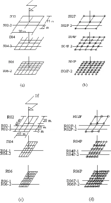
The characteristics of the grid are 50m*50m, and 75m*31.25m to achieve the equal area between two cases, the number of meshes is 16, the radius of the grid rods (r) is 0.005 m, the length of vertical rods (Lvr) is 2m, the radius of it (rvr) is (0.005m), the grid depth (h) is 0.5 m, the resistivity of the soil is 2000 ohm.m, and the total ground potential rise (GPR) is defined as 1V. The cases under study are shown in Figure 2.
Figure 3 illustrates the 3 dimensions (3D) and contour profile for the case R014P16.
It is clear that the ground potential rise (GPR) as well as distribution of the earth surface potential (ESP) during the current flow in the grounding system are important parameters for the protection against electric shock. The distribution of the earth surface potential helps us to determine the step and touch voltages, which are very important for human safe.
By definition, the touch voltage is the difference between the ground potential rise (GPR) and the surface potential at the point where a person is standing while at the same time having his hands in contact with a grounded structure, and the mesh voltage is defined as the maximum touch voltage to be found within a mesh of a ground grid. The maximum touch voltage is the difference between the GPR and the lowest potential in the grid boundary [1]. The maximum percentage value of Vtouch is given by
100
voltage%
Max touch
m in
GPR
V
V
grid t(1)
Where, Vgrid is the ground potential rise (GPR), which equal
the product of the equivalent resistance of grid and the fault
current and Vmin is the minimum surface potential in the grid
boundary.
Fig. 2: Grounding grids with different meshes and different locations of the vertical rods. (a. without vertical rods, b. with vertical rods at all point, c.
the vertical rods at the points across the diagonal and center lines, d. the vertical rods at the perimeter of the grid only)
Fig. 3: The distribution of EPS per GPR above the grounding grid (case R04P16 in two cases for rectangle and square grids)
Effect of the locations of the vertical rods on the grounding resistance and earth surface potential is presented in Figure 4.
0 50000 100000 150000 200000 250000
-50 0 50 100 150
E
S
P(
V
)
Distance along the diagonal of the grid from its center (m)
R04_4 R04P_4 R04P16_4
Fig. 4: The effect of vertical rod location on the earth surface potential for the case study of square grid
It is seen from Figure 4 that the minimum earth surface potential doesn’t vary significantly since the vertical rods are connected to grid in the homogenous soil. The vertical rods that connect to the grid should be used in the multi-soil to reach to the lower resistivity soil. In contrast the grid potential rise decreases considerably when the fault current is considered as 10kA. As a result the touch voltage decreases with increase the number of vertical rods to the grid at the same number of meshes. A small effect in the earth surface potential when changing the vertical rods locations at the same number of meshes then the economical cost plays a great part for choosing the suitable design for the square grids.
Figure 5 shows the variation of the touch voltage from the center of grid along the diagonal and it is clear that the maximum touch voltage is at the corner mesh of the grid at different soil resistivity.
Fig. 5: Variation of touch voltage from the center of grid along the diagonal case (R04P16).
Table I explains that if the number of meshes increases the grid resistance, step and touch voltages will decrease but we should take into account the total length of the conductors used in the grid (the cost of the grounding system), for example the case R08P gives us the good results but the length of copper used is 1062 m in this case, then the cost is much higher but we can choose the case R04P16 as the optimum case of design because it produces a suitable results and give economical cost.
TABLE I
GROUND GRID RESISTANCE, STEP AND TOUCH VOLTAGES AT DIFFERENT VERTICAL RODS LOCATIONS WITH GROUNDING
GRIDS [ IF= 1000 A]
Case lt (m) Rg
(ohm)
GPR (kV)
Vt max % of GPR
Vs max % of GPR
R02 300 23.1 23.1 41.4 17
R04 500 20.3 20.3 29 16
R08 900 18.6 18.6 20 12
R02P 318 22.7 22.7 40.9 20
R04P 550 19.9 19.9 28 16
R08P 1062 18.1 18.1 17.81 15
R08P57 1014 18.1 18.1 17.92 15
R02P08 316 22.7 22.7 40.92 18
R04P16 532 19.9 19.9 28 16
R08P32 964 18.2 18.2 18.08 15
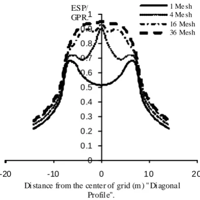
Figure 6 shows that an increase in the number of meshes makes the curve of earth surface potential much flatter and then a reduction in the grid resistance, touch and step voltages, also it is seen that the max touch voltage moves towards the corner mesh in the grid.
0 0.1 0.2 0.3 0.4 0.5 0.6 0.7 0.8 0.9 1
-20 -10 0 10 20
ESP/ GPR.
Di stance from the center of grid (m ) " Di agonal Profil e".
1 Me sh 4 Me sh 16 Mesh 36 Mesh
Fig. 6: Effect of the number of meshes on the earth surface potential
an important part to get the same results and decreases the cost of design.
The effect of profile location of the cases shown in Figure 7 will be studied.
Figures 8, 9 and 10 illustrate the effect of profile location, vertical rods and number of meshes for both earth surface potential and ground potential rise. It is noted that the number of meshes and the addition of vertical rods to the grid have a great effect for decreasing grid resistance and then both of ESP and GPR.
TABLE II
COMPARISON BETWEEN THE ADDITION OF VERTICAL RODS OR HORIZONTAL RODS TO A GROUNDING GRID
No of meshes 36 4
No. of vertical rods 0 9 Vertical rods length (m) 0 2 Total grid length (m) 140 78
Resistance (Ω) 4.26 4.29 GPR (V) at 100 A 426 429 Max touch voltage % GPR 25.0 31.1 Max touch voltage (V) 106.5 133.419 Max step voltage % GPR 16 16
It is seen from the results that the minimum earth surface potential doesn’t vary significantly when the number of meshes increases above 16 meshes, but in contrarily the grid potential rise decreases considerably. It is also seen in the pervious figures that the earth surface potential of 16 meshes is above that of 36 meshes because the profile location of the 16 meshes lies above one conductor of the grid which causes the earth surface potential is high in this region.
Fig. 7: Grounding grids with different profile locations. (a. square grids (20m*20m) without vertical rods, b. square grids (20m*20m) with vertical rods at all, , c. rectangle grids (10x40m) without vertical rods, d. rectangle
grids (10x40m) with vertical rods at all point)
Fig. 8: The earth surface potential (ESP) and ground potential rise (GPR) at specified profile location and different number of meshes, with and without
vertical rods for square grids
Fig. 9: The earth surface potential (ESP) and ground potential rise (GPR) at specified profile location and different number of meshes, without vertical
rods for square grids
Fig. 10: The earth surface potential (ESP) and ground potential rise (GPR) at specified profile location and different number of meshes, with vertical
rods for square grids.
Table III shows the values of ground grid resistance, step and touch voltages for the different profile locations of different configurations of grounding grids for fault current (If) of 100 A.
grounding systems. The profile location also plays a great deal for reducing the values of these parameters, the touch voltage decreases when the profile location comes near to the center line of grid.
TABLE III
THE EFFECT OF PROFILE LOCATION ON THE STEP AND TOUCH VOLTAGE FOR DIFFERENT RECTANGLE AND SQUARE GRIDS
Case R (ohm)
GPR (V)
Vsmax /GPR
Vtmax/ GPR
If at GPR=1 R02_1 2.273 227.34 0.096 0.2566 0.4398 R02_2 2.273 227.34 0.096 0.2918 0.4398 R02P_1 2.179 217.97 0.091 0.2567 0.4398 R02P_2 2.179 217.97 0.100 0.2751 0.4398 R04_1 2.079 207.94 0.091 0.1622 0.4808 R04_2 2.079 207.94 0.12 0.17 0.4808 R04P_1 1.965 196.56 0.073 0.1567 0.5087 R04P_2 1.965 196.56 0.093 0.168 0.5087 R06_1 2.004 200.47 0.099 0.1184 0.4988 R06_2 2.004 200.47 0.114 0.132 0.4988 R06P_1 1.868 186.85 0.082 0.116 0.5351 R06P_2 1.868 186.85 0.101 0.1162 0.5351 S02_2 2.626 262.68 0.111 0.3557 0.3806 S02P_2 2.491 249.16 0.1 0.336 0.4013 S04_2 2.363 236.30 0.144 0.1346 0.4231 S04P_2 2.20 220.07 0.133 0.1143 0.4539 S06_2 2.260 226.07 0.110 0.151 0.4423 S06P_2 2.072 207.28 0.096 0.1214 0.4824
3. FIELDCOMPUTATIONWITHEQUIVALENT
CHARGES
In the charge simulation method, the actual electric filed is simulated with a field formed by a number of discrete charges which are placed outside the region where the field solution is desired. Values of the discrete charges are determined by satisfying the boundary conditions at a selected number of contour points. Once the values and positions of simulation charges are known, the potential and field distribution anywhere in the region can be computed easily [15].
The basic principle of the charge simulation method is very simple. If several discrete charges of any type (point, line, or ring, for instance) are present in a region, the electrostatic potential at any point C can be found by summation of the potentials resulting from the individual charges as long as the point C does not reside on any one of the charges. Let Qj be a number of n individual charges and
Φi be the potential at any point C within the space.
According to superposition principle;
nj j ij i
P
Q
1
(2)where Pij are the potential coefficients which can be
evaluated analytically for many types of charges by solving Laplace or Poisson’s equations, Φi is the potential at contour (evaluation) points, Qj is the charge at the point charges.
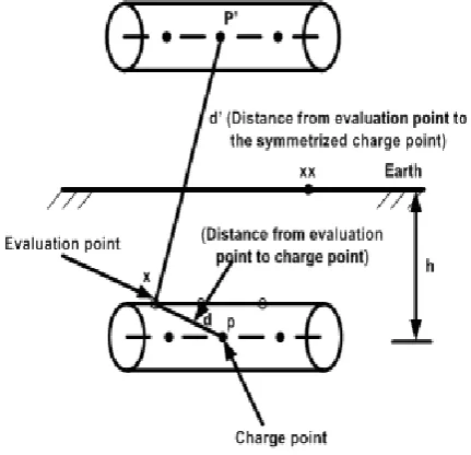
Because of the ground surface is flat, the method of images can be used with the charge simulation method and the potential will be characterized for being constant on the grounding grids and its symmetry [16]. The potential coefficients will be as in the following equation;
d
d
P
ij ij ij
'
1
1
4
1
(3)where, dij is the distance between contour point i and charge
point j and d’ij is the distance between the contour point i
and image charge point j’ as shown in Figure 11.
As in Figure 11, the fictitious charges are taken into account in the simulation as point charges. The position of each point charges and each contour point are determined in X, Y and Z coordinates where the distance between the contour (evaluation) points are calculated as the following ;
2
2
2i j i j i j
ij
X
X
Y
Y
Z
Z
d
Where, Xj, Yj and Zjare the dimensions of the point charge
and Xi, Yi and Zi are the dimensions of the contour point.
After solving 2 to determine the magnitude of simulation charges, a number of checked points located on the electrodes where potentials are known, are taken to determine the simulation accuracy. As soon as an adequate charge system has been developed, the potential and field at any points outside the electrodes can be calculated.
Fig. 11: Illustration of the charge simulation technique
The grid is divided into equal segments by the point charges distribution along the axis of grid conductors. Figure 12 shows the distribution of the point charges (dots) for the grounding grid (1 mesh), the number of point charges is distributed on the axis of the grid conductors equally and also the evaluation points distributed on each conductor as shown in Figure 12. The meshes of the grid are always symmetrical.
The charge simulation technique is used to get the ground resistance (Rg), ground potential rise (GPR) and then the
1
C
R
V
Q
C
g n j
j
(4)
where, V is the GPR that is defined 1 V, Qj is the charge of
point charge j that used for the calculation, ρ is the soil resistivity and ε is the soil permittivity.
In this section, some figures explain the earth surface potential along diagonal profile for the square grid with different number of meshes.
The characteristics of the grid are 50m*50m, the radius of the grid rods (r) is 8 mm, the grid depth (h) is 0.5 m, the resistivity of the soil () is 100 Ω.m, and the total ground potential rise (GPR) is defined as 1 V.
Figure 13 shows the Earth surface potential in 3D and the contour map of this case.
Fig. 12: Distribution of point charges on the grid (1 mesh)
Fig. 13a: ESP/GPR for 64 meshes
Fig. 13b: Contour map for 64 mesh grid
4. COMPARISONBETWEENTHEBEMANDCSM
The following case of study is taken to compare between the results by BEM and CSM, the input data about the grid configuration:
Number of meshes (N) = 64, side length of the grid in X direction (X) = 75 m, side length of the grid in Y direction (Y) = 75 m, grid conductor radius = 5 mm, vertical rod length (Z) = 0 (no vertical rod), depth of the grid (h) = 0.5 m, resistivity of the soil (ρ) = 2000 Ω.m and the permittivity of the soil is 9.
The following table I explains that the result from the proposed method is close to the other formula in [1] and also the values of resistance that calculated by [11-14].
TABLE IV
GROUNDING RESISTANCE BETWEEN THE BEM AND CSM AND THE OTHER FORMULAS THAT USED IN IEEE STANDARDS [1]
Formula R (Ω)
Dwight [1] 11.8
Laurent [1] 13.29
Sverak [1] 13.23
BEM [11-14] 12.67
Schwarz [1] 11.11
CSM 4320 Points 11.87
Figure 14 explains that the proposed method satisfies an agreement with the other method that used to calculate surface potential for example Boundary Element Method [11-14].
0 2 4 6 8 10 12 14
-150 -100 -50 0 50 100 150
E
S
P
(k
V
)
Distance from grid center (m)
BEM
CSM
Fig. 14: Comparison between proposed method and Boundary Element Method for 64 meshes grid
5. CONCLUSIONS
The vertical rods play an important role for reducing the grid resistance, the step and touch voltages. The number of meshes is an effective parameter for reducing the pervious values but it needs more copper then increases the cost. The study explains a small effect in the earth surface potential when changing the vertical rods locations at the same number of meshes hence the economical cost plays a great part for choosing the suitable design for the square grids, then the optimal case of the grids is that consists of 16 meshes with the vertical rods in the perimeter (case R04P16), it gives suitable results for the grid resistance, step and touch voltages and in the same time it presents an economical cost.
then the addition of vertical rods to the grounding grid gives a good performance and decrease the cost of design. Both vertical rods and number of meshes are considered effective parameters for reducing the grid resistance, the step and touch voltages. The paper demonstrates that another important parameter that effects in the pervious values is the profile location. The man location in case of fault determines the value of step and touch voltage that he will experiences. The figures illustrate that the dangerous point is at the side of the grid and comes in the corner mesh in the grid.
The proposed methods (BEM and CSM) that used to calculate the earth surface potential and grounding resistance due to discharging current into grounding grid are efficient. The validation of these methods is satisfying by a comparison between the results from it and the results from the formula in IEEE standard. The proposed methods give a good agreement with the IEEE standard. The two methods give the closest results to each other althought the different techniques that applied in each method.
REFERENCES
[1] IEEE Guide for safety in AC substation grounding, IEEE Std.80-2000.
[2] J. G. Sverak, “Progress in step and touch voltage equations of ANSI/IEEE Std. 80,” IEEE Trans. Power Delivery, vol. 13, no. 3, pp. 762-767, Jul. 1999.
[3] Sherif Salama, Salah AbdelSattar and Kamel O. Shoush, "Comparing Charge and Current Simulation Method with Boundary Element Method for Grounding System Calculations in Case of Multi-Layer Soil, International Journal of Electrical & Computer Sciences IJECS-IJENS Vol:12 No:04, pp.17-24, August 2012.
[4] Thinh Pham Hong ; Quan Do Van ; Thang Vo Viet “Grounding resistance calculation using FEM and reduced scale model” Electrical IEEE Conference on Insulation and Dielectric Phenomena, 2009. CEIDP '09, pp. 278-281, 2009.
[5] Salam, M.A. ; Ja'afar, S. ; Ariffin, M. “Measurement of grounding resistance by U-Shape and square grids”, TENCON 2010 - 2010 IEEE Region 10 Conference, pp.102-105, 2010.
[6] E. D. Sunde, Earth Conduction Effects in Transmission Systems, D. Van Nostrand Company Inc., New York 194, 1968.
[7] G. F. Tagg, Earth Resistances, Pittman Publishing Corporation, London, 1964.
[8] J. M. Nahman, V. B. Djordjevic, “Nonuniformity correction factors for maximum mesh and step voltages of ground grids and combined ground electrodes,” IEEE Trans. Power Delivery, vol. 10, no. 3, pp. 1263-1269, Jul. 1995.
[9] J. M. Nahman, V. B. Djordjevic, “Maximum step voltages of combined grid-multiple rods ground electrodes,” IEEE Trans. Power Delivery, vol. 13, no. 3, pp. 757-761, Jul. 1998.
[10] B. Thapar, V. Gerez, A. Balakrishnan, and D. A. Blank, “Simplified equations for mesh and step voltages in an AC substation,” IEEE Trans. Power Del., vol. 6, no. 2, pp. 601-607, Apr. 1991.
[11] I. Colominas, F. Navarrina, and M. Casteleiro, “Analysis of transferred earth potentials in grounding systems: A BEM numerical approach,” IEEE Trans. Power Delivery, vol. 20, no. 1, pp. 339-345, Jan. 2005.
[12] I. Colominas, F. Navarrina, and M. Casteleiro, "A boundary element numerical approach for earthing grid computation", Computer Methods in Applied Mechanics and Engineering, vol. 174, pp 73-90, 1990.
[13] I. Colominas, F. Navarrina, and M. Casteleiro, "A numerical formulation for grounding analysis in stratified soils", IEEE Trans. on Power Delivery, vol. 17, pp 587-595, April 2002.
[14] Colominas, I. ; Navarrina, F. ; Casteleiro, M. “Numerical Simulation of Transferred Potentials in Earthing Grids Considering Layered Soil Models”, IEEE Transactions on Power Delivery, Vol. 22, No. 3, pp.1514-1522, 2007.
[15] N. H. Malik, “A review of charge simulation method and its application,” IEEE Transaction on Electrical Insulation, vol. 24, No. 1, pp 3-20, February 1989.
[16] E. Bendito, A. Carmona, A. M. Encinas and M. J. Jimenez “The extremal charges method in grounding grid design,” IEEE Transaction on power delivery, vol. 19, No. 1, January 2004, pp 118-123.
BIOGRAPHIES
Sherif S. M. Ghoneim Received B.Sc. and M.Sc. degrees from the Faculty of Engineering at Shoubra, Zagazig University, Egypt, in 1994 and 2000, respectively. Starting from 1996 he was a teaching staff at the Faculty of Industrial Education, Suez Canal University, Egypt. Since end of 2005 to end of 2007, he is a guest researcher at the Institute of Energy Transport and Storage (ETS) of the University of Duisburg-Essen-Germany. In 2008, he got Ph.D Degree in Electrical power and machines, Faculty of Engineering-Cairo University (2008). He joins now the Taif University as an assistant professor in the Electrical Engineering Department, Faculty of Engineering. His research focuses in the area of high voltage engineering.