Edge Detection using Directional Filter Bank
S. Anand
Assistant Professor
Mepco Schlenk Engineering
College
Sivakasi
T. Thivya
P.G Student
Mepco Schlenk Engineering
College
Sivakasi
S. Jeeva
P.G Student
Mepco Schlenk Engineering
College
Sivakasi
ABSTRACT
Finding edges in digital images is an essential and important task in many imaging applications. This paper describes an edge detection using multi scale Directional Filter Bank (DFB). This method tries to solve two difficulties that edge finding algorithms must face: limited directions and combining the detected edges at different scales. The directional responses of DFB that represent the edge information can be used for edge detection. The steerable and scaled DFB has been presented to obtain directional along with scaled information. From the DFB based image decomposition, the scaled information is combined by scale multiplication. Finally, to evaluate edge detector performance the sensitivity, specificity, accuracy and Figure of merit ‘F’ parameters are used to compare with classical methods and the proposed approach provides better performance.
Keywords
Edge Detection, Directional filter bank, Scale multiplication
1. INTRODUCTION
Edge detection is an important tool in image processing in the field of feature detection and feature extraction. It is to simplify the image analysis by reducing the amount of data and preserving useful structural information. However, if the signal data is discrete, then the edges are often defined as the local maxima of the derivative(s). Essentially an edge detector is a high pass filter (operator) that can be applied to extract the edge points in a signal. There are classical 2-D gradient operators such as Roberts, Prewitt, Sobel and Fri-Chen for edge detection. All these operators being high pass filters are sensitive to noise. They are simple but limited in extracting the directional edge information due to separable implementation. In order to avoid this difficulty either 2-D non-separable filters or directional edge filters are used. To combat with noise, Marr and Hildreth operator is devised and these pre-smoothing approaches combine Gaussian smoothing while estimating gradient. They are useful in higher noise conditions and attractive due to low complexity linear implementation. The weakness of all above approaches is that the optimal result may not be obtained by using a fixed size operator.
Edges normally present not only single scale but also multiple scales. The developments in the field of multi-resolution wavelet transforms with their ability to detect and characterize singularities, attracted many researchers to explore the optimal edge detection problem in higher noise conditions. The advantage with multiscale approach is its inherent implementation, with variable size derivative operators at various scales, to tradeoff between detection and localization of local singularities. The indirect inter-dependence of wavelet coefficients at different scales opens the possibility to explore the hidden association of edge information at various scales (levels).
scales [1], multiscale products by Xu et.al. [2], is based on Rosenfeld’s idea of cross-scale correlation [3]. A few other multiscale singularity detection approaches are as [4]-[10]. However, the usefulness of wavelet based singularity detection is widely known from the literature; in general, wavelets have two limitations (i) isotropy and (ii) limited directions due to separable implementation. To analyze and represent an image, DFB can be employed and it can capture and represent signal singularities in the form of edges lying on smooth surfaces. Bamberger and Smith [11] proposed DFB for 2-D signals, and widely used in anisotropic multiresolution transforms found in [12-15]. Directional oriented representations of images are great interest for many years. Directional information is important in many image applications like image enhancement, denoising, edge detection and segmentation, classification and feature extraction. This paper proposes an approach to detect edges by using scaled version of directional filter bank which is applied in steerable manner. This provides directional specific information along with scale information.
2. DIRECTIONAL FILTER BANK
DFB is unique in their ability to decompose a multidimensional signal into several directional sub bands. Moreover, they are capable of frequency representation with high angular resolution and these properties make DFB more attractive. If the low pass and high pass filter response is given by using the poly phase filters P0 (ω) and P1 (ω). In
general, fan filter followed by a Checkerboard filter is implemented to obtain the wedge shaped frequency response. The wedge responses are useful to provide edge information and hence useful for our edge detection. Here P1 (ω) gives
edge information and a Checker board filter can defined by
c z1 , z2 =
1
2 P0 −z12 P0 −z22
− z0z1P1(−z12)P1(−z12)
Also P0(ω) and P1(ω) satisfy condition P0 (ω)2+ P1 (ω)2 =
1. The transfer function of the fan filter Fv(z1 , z2) is
obtained from the checkerboard filter.
Fv z1 , z2 =
1
2 P0 −z1z2 P0 −z1−1z2
− z21P1 −z1z2 P1 −z1−1z2
Ideal fan filter response is given by,
Fv ejω1 , ejω2
= c ej(ω1+ ω2)/2 , ej(ω1+ω2)/2
Figure 1 Frequency partitioning of DFB in 2D
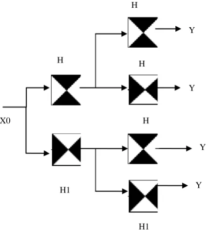
DFB is implemented at an n-level tree structured decomposition that leads to 2n sub bands with wedge shaped frequency partitioning. Figure.1 shows ‘3’ level tree structure and each sub bands corresponding to unique angular orientation. The block diagram of binary tree structure of the directional filter bank for two levels is shown in Figure 2. The input image is decomposed into 2n i.e. ‘4’ sub bands. The DFB allows for a different number of directions at each decomposition level and is designed to capture high frequency directionality of the coefficient. Low pass sub bands provide coarse acquisition and high pass sub bands should be able to extract directional information in an image. DFB is used to link the point discontinuities into a linear structure. The main advantage of designing the filter in frequency domain is that their frequency responses can be strictly beyond some critical frequencies.
The edges exist in an image at any scale and orientation. Thus, it is necessary to obtain the response of an edge filter at any arbitrary position and orientation. Steerable Filters are such filter and tuned to get possible orientation. One method to find the response at many orientations is to apply many versions of the same filter each different from the others by a small rotation in angle. A more efficient approach is to apply a few filters corresponding to a few angles and interpolate between the responses. Arbitrary orientation of steerable filter can be synthesized as a linear combination of a set of basis filters.
Figure 2 Block diagram of DFB
The simplest illustration of the steerable principle is the directional derivative of a two-dimensional function, G(x, y). The directional derivatives of that function (in polar coordinates) in ‘0𝑜’ and ‘90𝑜’ orientations are:
G10 r, θ = cos θ G(x, y)
G1π/2 r, θ = sin θ G(x, y)
Where the subscript indicates the order of the derivative, and the superscript indicates the angle of the derivative direction. It is straightforward to show that the function G1 can be edge
filter and can synthesize at an arbitrary orientation ‘ ’ using the equation:
G1ϕ r, θ = cos ϕ G10 r, θ + sin ϕ G1π/2 r, θ
The directional derivative G1 can be generated at an arbitrary
orientation as a linear combination of the basis filters G10and G1π/2, where the coefficients cos ϕ and sin ϕ
are referred to as the interpolation functions. Our contribution is to directly use G(x, y) as a simple 2D directional filter to obtain the edge response. In other words any 2D directional filter can be steerable operated to get the edge responses at various directions.
3. DFB BASED EDGE DETECTION
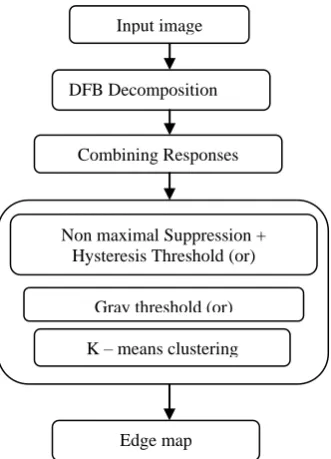
Figure 3 shows the block diagram of the proposed methodology. In this paper it is been described that the input image is decomposed using the DFB. This provides directional specific information and it is subjected to various edge labeling algorithms to obtain the edge map more effectively. Following are some edge labeling techniques used to obtain the final edge map.
8
6
7
5
2
4
6
7
8
1
2
3
4
5
3
1
Y 1
Y 3
Y 4
H1 H 0 H 1 H
0
H1 X0
Figure 3 Block diagram of the proposed method
3.1 Non Maximal Suppression (NMS)
This has the effect of suppressing all image information that is not a part of local maxima. Given estimates of the image gradients, a search is then carried out to determine if the gradient magnitude assumes a local maximum in the gradient direction. The image is scanned along the image gradient direction, and if pixels are not part of the local maxima, they are set to zero. This is followed by hysteresis threshold (HT) to remove noisy local maxima in NMS. Proper threshold preserves connectivity of contours. This uses two thresholds - the lower threshold and the upper threshold.
3.2 Gray Threshold
The gray threshold is the simplest and most widely used threshold method. It computes a global threshold that can be used to convert an intensity image to a binary image. This technique uses Otsu's method, which chooses the threshold to minimize the intra class variance of the black and white pixels.
3.3 K means Clustering Algorithm
In this approach, set of input parameters are partitioned into K clusters, where K is known in advance. This method is based on the identification of centroids each K- clusters. Thus instead of computing the pair wise inter pattern distances between all the clusters, here the distances may be computed only from the centroids.
4. RESULTS AND DISCUSSIONS
4.1 Edge detected results
The proposed method has been tested on standard test images like the ‘home’ image of size 256 x 256, ‘leaf’ image of size 592 x 896 and ‘cameraman’ image of size 256 x 256. In order to evaluate the performances, the airplane image and its corresponding ground truth image of size 409 x 659 is considered. The images are taken from the USF (University of South Florida) image database, USC-SIPI (University of South California-Signal and Image Processing Institute) and Caltech database. The image is convolved with the Directional filter bank and for example, two filter coefficients are given below.
H1=
0 0.1414 0.2828 0
−0.2828 −0.5657 0.5657 −0.2828
0 0.2828 −0.1414 0
H1=
0 0 −0.0625 0 0
0 −0.1250 −0.2500 −0.1250 0
−0.0625 0 0
−0.2500 −0.1250
0
1.7500 −0.2500 −0.0625
−0.2500−0.1250 0
−0.625 0 0
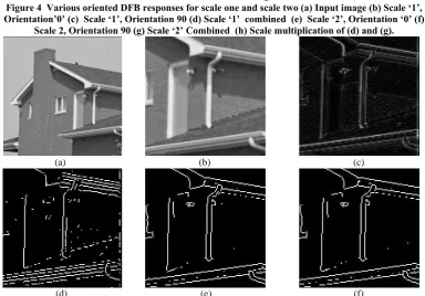
The decomposed images at various directions and scales using
𝐻1are shown in Figure 4. In this paper, we consider two
scales for edge detection. Figure 4 shows various orientations with DFB responses for first and second scales. The rotated 2-D 2-DFB coefficient matrix is convolved with original image to get the various oriented responses. They are shown in Figure 4(b)-(d). The second scale contains broader edge information and it is less prone to noise whereas first scale contains thin edges. The directional responses of both the scales are combined using scale multiplication. The purpose of combining two scales is to suppress noisy components and to enhance the edge information. The combined two scales edge information is shown in Figure 4(h).
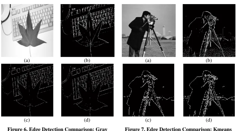
Figure 5 shows the comparison of edge detection using NMS and HT with conventional operators. Figure 5(a) shows the input image and Figure 5(b) is the image area cropped from the original image. A part of the original image is cropped to show the effectiveness of the proposed methodology clearly. Figure 5(c) shows the scale one and scale two combined image. Figure 5(d) shows the edge labeled on Figure 5(c) using NMS followed by HT and is compared with classical Sobel and Prewitt operator as shown in Figure 5(e) and 5(f) respectively. From the Figure5 it is observed that the roof walls are detected well by using the proposed methodology than the conventional Sobel and Prewitt operator. Figure 6 compares gray threshold on DFB edge information of ‘leaf image’ with other methods. From the Figure 6 it is observed that the leaf veins are detected more clearly in proposed methodology than Sobel and Prewitt operator.
Combining Responses DFB Decomposition
Edge map Input image
Non maximal Suppression + Hysteresis Threshold (or)
Gray threshold (or)
(a) (b) (c) (d)
(e) (f) (g) (h)
Figure 4 Various oriented DFB responses for scale one and scale two (a) Input image (b) Scale ‘1’, Orientation’0’ (c) Scale ‘1’, Orientation 90 (d) Scale ‘1’ combined (e) Scale ‘2’, Orientation ‘0’ (f)
Scale 2, Orientation 90 (g) Scale ‘2’ Combined (h) Scale multiplication of (d) and (g).
(a) (b) (c)
(d) (e) (f)
(a) (b) (a) (b)
(c) (d) (c) (d)
Figure 6. Edge Detection Comparison: Gray Threshold (a) Original Leaf image (b) Proposed
method (c) Sobel (d) Prewitt.
Figure 7. Edge Detection Comparison: Kmeans (a) Original Cameraman image (b) Proposed
method (c) Sobel (d) Prewitt
Figure 7 compares k means on DFB edge information of ‘Cameraman’ with other methods. From the Figure 7 it is observed that the edges are detected more clearly in proposed methodology than Sobel and Prewitt operator.
4.2 Performance Comparison
In this section, we compare the performances of the edge detection of our methodology using various techniques with that of the conventional edge detectors like Canny, Sobel, Prewitt. In our experiments, the canny edge detector uses two thresholds; lower threshold and upper threshold as 0.1 and 0.25 respectively.
The standard deviation is set to one. The optimal setting is made according to the canny method in [16] that is being used in our experiment. We choose sensitivity, specificity, accuracy as described in [17],[18]. and Figure of Merit ‘F’ parameters [19] to measure the performance. For every pixel in an image there are four possible edge detection results.The edge pixel is compared with the ground truth image to detemine the accuracy, sensitivity, selectivity in terms of the results namely true positive (TP), false positive (FP), true negative (TN), false negative (FN).
(a) (b)
Figure 8 (a) Original image (b) Corresponding ground truth TP - Edge pixel in an image is detected correctly as an edge
pixel, FP - Non edge pixel is detected wrongly as edge pixel, TN - Non edge pixel detected correctly as non edge pixel, and FN - Edge pixel detected wrongly as non edge pixel. The true positive rate (TPR) or sensitivity is given by TPR = TP +FNTP . False positive rate(FPR) is defined as FPR = FP +TNFP . True negative rate (TNR) or Specificity is given by TNR = 1 −
FP. Accuracy in percentage is obtained by ACC =
TP +TN
TP +TN +FP +FN× 100. The Pratt’s Figure of merit (F) is given
by which is 𝐹 = max Ni,Na 1 Ndk=11+∝d12(k). where EI and ED
are the number of ideal and detected pixels, respectively, d2(i) distance between detected and ideal pixels and α is the scaling constant and set at 1/9 in this experiment. Figure 8(a) and 8(b) shows the original and the corresponding ground truth from the USF dataset is used to compute the performance paprametrs. The quantitative performance comparisons are
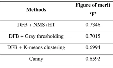
Table 1: Figure of merit
Table 2: Comparison between proposed methodologies with conventional edge operators
We can see that the accuracy of the proposed methodology is higher compared to the conventional edge detectors and also the sensitivity is also low and the specificity is high compared to other classical edge detectors hence providing better performance in terms of accuracy. Also the figure of merit of the proposed methodology is better than the canny operator.
5. CONCLUSION
In this paper, we have proposed the directional filter bank for edge detection which is useful in capturing and representing edges in various directions and scales. This approach helps in providing directional specific information along with scale, hence collecting more information. This study compares the work with that of Sobel edge operator and Prewitt edge operator. In addition, our proposed methodology has provided better results in terms of accuracy, sensitivity, specificity, and Figure of merit. From the results it is observed that the proposed method for edge detection provides a better result and acts as the good method of extracting the information
6. REFERENCES
[1] Mallat. S and Hwang. W L. 1992. Singularity Detection and Processing with Wavelets. IEEE Trans. Info. Theory, 617-643.
[2] Mallat S. and Zong S. 1992. Characterization of Signals from Multiscale Edges. IEEE Trans. PAMI, 14, 710-732.
[3] Xu Y. Weaver J., Healy D., and Lu J. 1994. Wavelet Transform Domain Filters: A Spatially Selective Noise Filtration Technique. IEEE Trans. Image Proc. 3, 747-758.
[4] Rosenfeld A. and Thurston M. 1970. Edge and Curve Detection for Visual Scene Analysis. IEEE Trans. Computer, 20, 562-569.
[5] Sadler B M., Pham T. and Sadler L C. 1998. Optimal and wavelet based Shock Wave Detection and Estimation, J Acoust. Soc. Am., 104(2), 955-963.
Methods Figure of merit
‘F’
DFB + NMS+HT 0.7346
DFB + Gray thresholding 0.7015
DFB + K-means clustering 0.6994
Canny 0.6592
Methods
Parameters
DEB + NMS + HT
DFB + Gray threshold
DFB +
K-means Sobel Canny Prewitt
TP 1519 1576 1436 2878 2803 2886
FN 5679 5628 5762 4320 4395 4312
FP 6169 8205 7304 11737 12354 11563
TN 256164 254128 255029 250596 249979 250770
TPR
(Sensitivity) 0.2110 0.2181 0.1995 0.3998 0.3894 0.4009
FPR 0.0235 0.0313 0.0278 0.0447 0.0471 0.0441
TNR
(Specificity) 0.9765 0.9687 0.9515 0.9553 0.9529 0.9559
Accuracy
[7] Park D J., Nam K N., and Park R H. 1995. Multiresolution Edge Detection Techniques. Pattern Recognition, 28(1), 211-219.
[8] Shun-feng Ma ; Geng-feng Zheng ; Long-xu Jin ;Shuang-li Han ; Ran-feng Zhang, 2010. Directional multiscale edge detection using the contourlet transform, Advanced Computer Control (ICACC).
[9] Chen Jinlong ; Zhang Bin ; Qi Yingjian ; Jin Fei ; Si Xuan, 2010. Image Edge Detection Method Based on Multi-Structure and Multi-Scale Mathematical Morphology, Multimedia Technology (ICMT).
[10]Anand S and Jayasudha N. 2011. Edge detection using Surfacelet Transform, International Journal of Image Processing and Application, Vol.2, No.1.
[11]Roberto H. Bamberger and Mark J. T. Smith. 1992. A filter Bank for Directional Decomposition of Images: Theory and Design. IEEE Trans on Signal processing, Vol.40, No: 4.
[12]Javad Museve Niya and Ali Aghagolzadeh. 2004. Edge Detection using Directional Wavelet Transform. IEEE Melecon.
[13]Minh N. Do and Martin Vetterli. 2005. The Contourlet Transform: An Efficient Directional Multiresolution Image Representation. IEEE Trans. On Image Processing, Vol. 14, No. 12.
[14]Arthur L. da Cunha, Jianping Zhou and Minh N. Do. 2006. The Nonsubsampled Contourlet Transform: Theory, Design, and Applications. IEEE Trans. on Image Processing, Vol. 15, No. 10.
[15]Yue Lu and Minh N. Do. 2007. Multidimensional Directional Filter Banks and Surfacelets. IEEE Trans. on Image processing, Vol: 16, NO: 4.
[16]Sheng Yi, Demetrio Labate, Glenn R. Easley, and Hamid Krim. 2009. A Shearlet Approach to Edge Analysis and Detection. IEEE Trans. on Image Processing, Vol. 18, No. 5.
[17]Canny J. 1986. A computational approach to edge detection. IEEE Trans. Pattern Anal. Mach. Intell., vol. 1–8, no. 6, pp. 679–698.
[18]Bowyer K., Kranenburg C., and Dougherty S. 2001. Edge detector evaluation using empirical ROC curves. Computer. Vision. Image Underst., Vol. 84, no. 1, pp. 77–103.
[19]Wei Jiang, Kin-Man Lam, and Ting-Zhi Shen. 2009. Efficient Edge Detection Using Simplified Gabor Wavelets. IEEE Trans. on Systems, Man, and Cybernetics- Part B: Cybernetics, Vol. 39, No. 4.