Self-Driving Car Model–Brute Force Approach using Monocular Vision and Transfer Learning on Unmarked Roads

Self-Driving Car Model–Brute Force Approach

using Monocular Vision and Transfer

Learning on Unmarked Roads

Mayank R. Vanani

Dept. of Instrumentation and Control Engineering, Nirma University, Ahmedabad, Gujarat, India

Abstract

Artificial Intelligence has spurred the advent of self-driving cars. Commercially viable autonomous cars inculcate lot of complex sensors in order to perceive the world. These cars are built for more standardized road conditions with distinct features. So, this paper cites an approach undertaken to suit more mercurial environment. A children’s toy car is used to maneuver over the university campus road which is built of Reinforced Cement Concrete (RCC) and has very few features that too with subtle difference. Environmental noise like shadows and varied day-lighting condition posits a grim challenge. A real-time system is built with algorithmic software driven approach. Also, brute logic is coded to mimic the behavior of actual self-driving car. For example, gradual acceleration, gradual braking, sudden braking in case of emergency. Concepts of Pulse Width Modulation (PWM) have been utilized to control the acceleration-velocity dynamics of car. Transfer Learning is used to classify and detect obstacles in the path and algorithm is written to aid subsequent decision making. Overall, a rather brute force algorithmic approach is used to build this real time system.

Keywords

Transfer Learning, Deep Learning, Adaptive Cruise Control, Real-Time System, Region of Interest (ROI)

I. Introduction

The advancement in Artificial Intelligence field has spurred the inevitable advent of autonomous systems. Deep Learning has been instrumental in the notion of perception of world by machines. Whereas software algorithms have made it possible to crunch complex problems to mere few lines of code to make such autonomous system more efficient and fool proof. One such field of active research is Self-driving car. A self-driving car is junction of various systems like adaptive cruise control achieved with help of IR array, lane assists which uses proximity sensors, parking assistant with the use of computer vision and distance sensors, classification of obstacles by use of deep learning techniques. Commercially available self-driving cars make the use of 3D camera or LIDAR for better perception of world because along with visual graphics, it is able to gather depth information with the use of Point-Cloud [1]. More and more sensors are deployed in order to avoid the accidental scenarios and to make the system more reliable. In this thriving field of robust advancement, one approach that has been cited in this paper is of more software-logic based approach. It becomes objective when designing autonomous car for standard lanes as the features are definitive – black roads, white lines, yellow foot lanes. But when the environment changes to a more rural setting like University Road - it becomes a complex problem with very less identifiable features and the added noise. Simple Computer Vision technique render useless for such settings. To mitigate it, hard-coded algorithm is devised to control the car dynamics and it sits on top of AI algorithm that detects obstacles and further decision is taken as per the developed algorithm.

II. Proposed Objectives

The idea is to build a working model using electronics and software systems to meet the following key points:

Obstacle avoidance using IR sensors •

Adaptive Cruise Control •

Steering advice using Computer Vision •

Object detection and classification using Convolutional •

Neural Networks

Depth estimation using bounding box generated around •

classified object.

III. Car Components

Children’s toy car – approx. 100cm by 70cm •

Small range sharp IR -GP2Y0A02YK0F(20cm –150cm); •

Long range IR GP2Y0A0710K0F (100cm – 550cm) •

Logitech Camera – C310 HD CAM •

‘Robokits’ make Motor Driver – 20A •

DC motors – 12V, 25W •

Arduino MEGA 2560 •

GPU – Nvidia 940 MX (inbuilt in laptop) •

Battery – AC Delco 9 Ah •

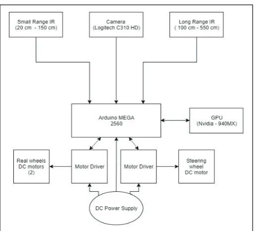
IV. Car Architecture

A toy car with inbuilt 3 DC motors – 2 for rear wheels and 1 for steering is used. 2 IR sensors are placed on the bonnet, in front-central part with 5cm distance apart which is minimum distance for interference-free operation (experimentally obtained). Logitech Webcam is placed just behind the IR sensors, on the bonnet on a raised platform. Rest of the circuitry consisting of motor drivers, Arduino, GPU and Battery rest at the back of the car. A schematic block diagram of component connection is given below in fig. 1.

V. Adaptive Cruise Control

Adaptive Cruise Control (ACC) is vital for a self-driving car. It is a method that has evolved out of cruise control. Cruise Control is an autonomous feature that maintains the car at a fixed desired speed. This feature is particularly useful for long drives where the roads are fairly wide and has less vehicles. ACC takes this system up a notch. In this feature, car adjusts its speed along the way according to traffic. An upper limit is specified for the maximum speed. Within this range, the car adjust its speed based on the distance of the vehicle or obstacle in front of it.Thus, maintain a safe distance and exempting the driver from frequent acceleration and braking. This feature is particularly useful in roads with heavy traffic [2-3].

So, ACC was achieved in two stages. IR sensors and Computer Vision was used to articulate a fool proof system.

A. IR Sensor Array

The IR sensor array for this system consisted of two Infrared Sensor of different range. Short range IR (20cm – 150cm) and long range IR (150cm – 550cm) together constitute a range of available control of 20cm to 550cm. Added advantage of using a short range IR is that we get higher precision of obstacle distance when the object is closer to car. So, now different zones are classified as shown in the fig. 2 and its associated speed is mapped and hard coded.

Fig. 2: Zone Classification for Combined IR Sensor Array

At first, the program is written in Arduino which is readily available microcontroller and has user-friendly hardware interface. So the program is written in Arduino IDE and is then uploaded into its RAM. Pulse Width Modulation is a technique in which digital signal’s amplitude is varied to vary the output power to the PWM-supplied device [4]. So as per the image, as the object gets closer to the car, less power is supplied to the motors and hence speed of car reduces.

Since, the code was taking a huge time, shifting the code base to embedded C proved to be of huge upgradation. The latency of single loop reduces to mere 3 milliseconds. Hence, it fetches an average of 300 IR pings per second. This improves the response time of the system. Also, sudden changes in output power using PWM may harm the battery and motor life. To mitigate this problem, small PWM factor is fine-tuned according to this model.

B. Computer Vision

Camera is used to aid the ACC that is achieved using IR sensors [5]. Since, not all objects in front of car are of our interest, it is better to ignore them. So, only those objects that fall in the ‘Region of Interest’ (ROI) are considered in the path of the vehicle and subsequently along with using computer vision technique of object tracking, IR sensor based algorithm is activated to track its physical distance from the car. This is further elaborated in ‘Computer Vision Module’ section of this paper.

VI. Stabilized Discrete Steering Advice

Steering position in car is discrete. This is due to the fact that the car has inbuilt DC motor used for steering. Amount of rotation cannot be controlled in DC motor as in servo motor.Hence, time based control is adopted to control the rotation of steering wheel. There are 7 different position that steering wheel could rest in. One in the centre, 3 on right and 3 position on left. The steering wheel is operated by DC motor which in turn is operated by motor driver. The motor driver receives signals from computer vision algorithm that is responsible for edge detection and obstacle classification.

A. Lane Marking Technique

One of the crucial element for guiding the autonomous vehicle is the environment. It needs to distinguish traversable path from non-traversable regions. The environment for which the system is built is more of rural setting. This car is built to run on university campus road which is made up of Reinforced Cement Concrete (RCC). It is 15ft road with concrete bricks making the edges. Since the road and edges are of same colour – grey, it posits a problem to identify the edges distinctly so as to keep the car in between the edges and eventually in between the road.

Adding to it, the illumination also varies throughout the day time. Since, computer vision algorithms are heavily dependent on lighting condition, simple techniques cannot not be used to get the edges [6].

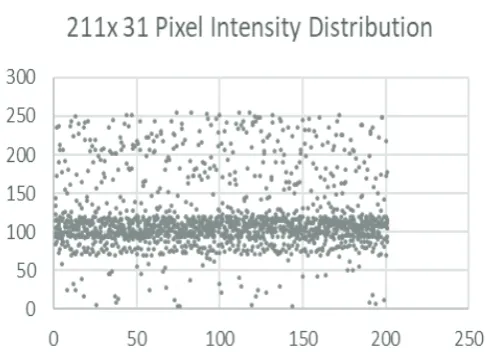
Hence, pixel-value based approximation is used to identify the edges. This is a peculiar approach that is suited for this campus road or similar conditions only. Here, a video sample of the campus road was collected for different day times. Then, pixel values were monitored and recorded for grey-scaled frames in a database for a small window of 211px by 31px that contained the edges. The scatterplot obtained was plotted as below.

Also histogram espoused the fact that edges pertained pixels values ranging from 90 to 120 for a grey-scaled image. So, two side lines (marked in red in fig. 5) are placed on the frame to monitor the pixel values. These are 300px by 1px. As it gets the 3 consecutive pixel values within this range, it means that edges are identified and the red slider on each side lines move to that pixel. The position of these red sliders are recorded for further calculations.

Fig. 4: Histogram of the pixel distribution obtained from fig. 3.

Fig. 5: Edge sliders (red) and steering marker (blue) in 960px by 540 px

B. Stabilized Steering

Although, various steering approaches have been devised, this projects utilizes the use of lane marking technique extensively to steer in order to eliminate additional computational cost [7]. As we get the location of edges with the help of marker, we calculate the mean of the distance along the x-axis. The calculated mean is then subtracted from the center position to get the net change in the direction of car that is required from the center which in turn was subtracted from previous counter to get the total change of steering that the car must undergo from the current position it is in. Mathematically, it can be represented as follows -

One of the biggest challenge was the high frequency fluctuation of steering wheel. As the car moves with an average pace of 4kmph, number of frames processed per second were 12. So when the car was running in center, there was heavy updating of steering wheel’s position which was although remaining in the center, but continuously swaying left and right with minute ∆steering value. So, there is a need to smoothen out the steering motion to make it more lucid.Although, Model Predictive Control [8-9] is a great strategy to implement as a solution, but since it’s computationally expensive in terms of loss of frames per second, it is not deployed in this project. Rather, a more brute force approach is utilized to preserve the current rate of frame processing power which is 19fps. Hence, 6-point monitoring is used to stabilize the ∆steering. The suggested ∆steering value and previous five values are monitored and if the suggested value is within ±0.5 Standard Deviation, then the value is parsed as effective steering value to be appended and the action is taken by issuing signal to the motor driver to rotate the steering wheel. The stabilized steering value is obtained with the help of this approach. The graph below depicts the trajectory of car on straight path.

Series 1 (blue): steering without stabilization

Series 2(red): steering with 6-point monitoring stabilization

Fig. 6: ∆steering Representing Trajectory of car on Straight Path

VII. Computer Vision Module

Monocular camera is used to perceive the surroundings. There are sophisticated cameras with better resolution, but reason for using this is just to check the extent of accuracy that we can get by software. For this model, Logitech 310 HD Webcam is used as it has a feature of 720p recording. The frame size reduced to 940 by 540 pixels.Then it is gray-scaled to make the processing less computational as it is easy to process single value of an individual pixel rather than 3 values for a single pixel in RGB values.

A. Object Detection using Transfer Learning

Transfer Learning is a methodology in which pre-trained model can be imported to suit to any problem set with similar application of classification of objects. If new objects are to be learned by the model, then the final weights of pre-trained models are used as starting weights for new application.

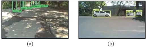
Tensorflow Object Detection API is a tool used for transfer learning [10]. In this context, “ssd_inception_v2_coco” model was used. Single Shot Detector (SSD) is an algorithm that unlike other computationally expensive algorithms, omits pixel resampling. Thus bringing tremendous improvement in speed and works with good amount of accuracy even for low resolution images. Inception model fetches very good amount of accuracy and stability of bounding boxes. Earlier less computational “ssd_mobilenet_v1_ coco” was used. However, the bounding box fluctuated heavily. Hence, it became hard to track and assure the presence of obstacle in the path of car. Hence, experimentally deploying various models trained on “Common Objects in Context” (COCO) dataset, inception model proved to give best results. In all these models, accuracy came at cost of computing. Hence it is a trade-off that one can decide as per the system in hand.

Further, the COCO dataset has 80 classes of pre-classified objects of “things”. Of these, most of the objects that the car encountered on the college campus were already present among them such as vehicles, people and animals. Hence 23 classes of 80 were retained, while deleting the rest. Hence this also improved frames processed per second.

(a) (b) Fig. 7: Real-time Output of Classifier on Campus Road

B. ACC and Obstacle Avoidance Algorithm

As shown in the fig. 8, the blue box represents the ROI which is hard-coded. So, after bounding box is drawn around the classified object, perspective transform is applied on the frame. Then the y-axis pixel distance of the bottom edge of the bounding box is recorded and its vertical distance from the bottom edge of the frame is calculated. This is then parsed through an equation that maps this calculated pixel distance to actual distance. This equation is obtained empirically by recording data by keeping the objects at different known distance from the car and then getting the pixel distance of its bounding box’s bottom edge to bottom edge of 950px by 540 px frame. Then simple polynomial fitting of the curve suffices for nearly accurate result.

Fig. 8: Hard-coded coordinates of ROI in 960px by 540px frame.

Now, as the classified object falls inside the ROI, its zone isrespectively reported. ROI is divided into 3 horizontal zones stacked on top of each other i.e. based on vertical distance or y-axis pixel distance (refer fig. 9):

(300 – 400) → “Object in Vicinity” •

(401 – 500) → “Warning” •

(501 – 540) →“Collision Warning” •

When the classified object falls in the zone of “Warning” and “Collision Warning”, IR sensors are activated to get the physical feedback of the distance of the object as calculated from the mapped polynomial algorithm. Hence, two-layer system is used to confirm the presence of obstacle in the path way of car and subsequently take the steering decision. If there is sufficient space between the road edge and the obstacle, then the car steers past it. If there is no gap, then the car gradually slows down until it stops at safe distance to the object. If the detected obstacle moves out of ROI, then the car gradually picks up to achieve its maximum speed.

Fig. 9: Zone classification of ROI

VIII. Result

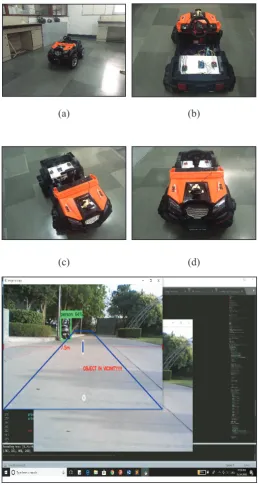
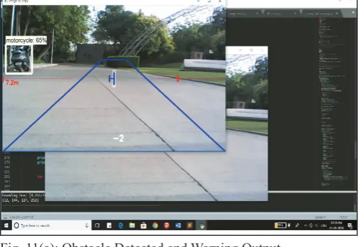
With the use of IR sensors and computer vision, a self-driving car was able to maneuver on campus road. Steering advice was stable and did not experience any sudden jerks. Since the car had wheels that were rugged for more grip to the ground, the camera feed had wavy nature. This is stabilized by resting the camera on thermocol which act as cushion. The classifier is able to detect objects in the frame and give steering advice and changes the speed if it falls inside the ROI. On straight path, the motion of car was fairly straight. Also during turn, camera aperture created fall short to capture the edges of the road. Hence, contained wavy motion at turns but not once did it collided with the edges. Further, the inception model was trained to identify campus road signs. Since the accuracy was not great enough, the feature was just passively implement i.e. it detects road sign but no actions are taken in response to it. The hardware implementation is given in fig. 10 and the output screen obtained after applying computer vision techniques is shown in fig. 11.

(a)

(c)

(b)

(d)

Fig. 11(a): Obstacle Detected and Warning Output

Fig. 11(b): Steering Output and Object Monitoring

IX. Acknowledgement

I would like to thank Prof. Vishal Vaidya who has been my mentor and guide for this project. Prof Vishal Vaidya is working as an Assistant professor, in the department of Instrumentation and Control engineering, Institute of Technology, Nirma University. He has more than 10 years of experience in the field of Teaching and Research. He obtained his BE in Instrumentation and Control Engineering and ME in Applied Instrumentation from the Gujarat University in the year 2004 and 2014 respectively. He has published research papers in the area of Robotics, control and embedded applications in International Journals and International conferences. He has guided many UG dissertations based on robotics and artificial intelligence. He has served as the member of Board of Studies. He is currently pursuing PhD at Gujarat Technological University. His area of interest are robotics and control, A.I algorithms for learning robots.

References

[1] F. Leberl, A. Irschara, T. Pock, P. Meixner, M. Gruber, S. Scholz, A. Wiechert,“Point Clouds: Lidar versus 3D Vision”, Photogrammetric Engineering and Remote Sensing, 2010. [2] Rohan Kumar; Rajan Pathak; “Adaptive Cruise Control –

Towards a Safer Driving Experience”, IJSER, Vol. 3, Issue 8, 2012.

[3] V.V. Sivaji, Dr. M. Sailaja,“Adaptive Cruise Control Systems for Vehicle Modeling Using Stop and Go Maneuvers”, IJERA, Vol. 3, Issue 4, 2013.

[4] [Online] Available: https://www.electronics-tutorials.ws/ blog/pulse-width-modulation.html

[5] Miguel Angel Stelo, Jose E Naranjo, Carlos Gonzales; “Vision based Adaptive Cruise Control for Intelligent Road

Vehicles”, IEEE/RSJ International Conference on Intelligent Robot and Systems, 2018.

[6] Graham D. Finlayson,“Color and illumination in computer vision”, The Royal Society Publishing, 2018. [Online] Available: https://doi.org/10.1098/rsfs.2018.0008

[7] Jarrod. M. Snider,“Automatic Steering Methods for Autonomous Automobile Path Tracking”, Robotics Institute, CMU, 2009

[8] Kai Liu, Jianwei Gong, Shuping Chen, Yu Zhang, Huiyan Chen; “Model Predictive Stabilization Control of High-Speed Autonomous Ground Vehicles Considering the Effect of Road Topography”, applied science, MDPI, 2018. [9] “MPC-Based Approach to Active Steering for Autonomous

Vehicle System”, [Online] Available: https://borrelli. me.berkeley.edu/pdfpub/pub-6.pdf

[10] [Online] Available: https://medium.com/object-detection- using-tensorflow-and-coco-pre/object-detection-using-tensorflow-and-coco-pre-trained-models-5d8386019a8