Analysis of Motion Velocity in Ultrasound Images

(1)



Abstract— In this paper, block-matching with Gaussian Filter

adaptive technique is proposed to estimate the motion velocity displacement point in the ultrasound image. We apply the Hexagon-Diamond Displacement Point (HDDP) technique to estimate the motion displacement. The motion displacement is based on the hexagon and diamond displacement pattern search points. The displacement pattern search point is to determine the displacement of motion velocity point in the ultrasound image sequence. The motion velocity displacement point is then used as reference point to access the diagnose or problematic area. Furthermore, motion velocity displacement point will be used as reference point to measure the displacement distance from the original point. At the same time, Gaussian Filter will help to suppress the existing high level of noise in order to improve the point signal-to-noise ratio (PS NR) of the ultrasound image sequence. The experimental result shows that the Gaussian Filter helps to improve the PS NR points in the ultrasound images sequence.

Index Term— Hexagon Pattern, Diamond Pattern,

Displacement Point, Gaussian Filter, 8



8 Block-Based I. INTRODUCTION

Motion velocity displacement analysis is useful in medical imaging as a diagnose tools [1-3]. Motion velocity displacement [4] also can be used for image sequence compression using block based motion estimatio n technique. Several techniques using the optical flow motion estimation has been studied extensively using image sequences and many algorithms continue to be developed [5-9]. Optical flow estimation [10-11] is conducted, for example, to improve the efficiency of encoding image or to enhance the display or movement of some particular area of the image [11]. Motion measurements are also used in breast deformation analysis to measure the elastic properties of tissues and to provide an indication of tissue hardness by computing a strain image or relative Young’s modulus image [12].

Kontogeorgakis et al. [13] estimated the motion between

T his work is supported in part by Universiti T eknikal Malaysia Melaka under Grant PJP/2009/FKEKK(10D)S546 .

Ranjit Singh Sarban Singh, Ahamed Fayeez T uani Ibrahim, and Sani Irwan MD Salim is attached with the Computer Deparment, Faculty of Electronics Engineering and Computer Engineering. Engr. Siva Kumar Subramaniam is attached with the Industrial Electronics Department,

Faculty of Electronics Engineering and Computer Engineering in Universiti T eknikal Malaysia Melaka (UT eM) phone : +606-5552161,

fax: +6065552112; (email: ranjit.singh@utem.edu.my, email: fayeez@utem.edu.my, email: siva@utem.edu.my, sani@utem.edu.my).

blocks of ultrasound images using the Minimum Absolute Difference (MAD) of their luminance values in order to

estimate a motion-magnitude map. Yeung et al. [14] estimated

motion in ultrasound sequences by block-matching with the Sum of Absolute Differences (SAD) used as the matching

criteria. In year 2004, Behar et al. implements the

block-matching technique using ultrasonic images to estimate the heart translation based on region of interest area [15]. Block-matching technique is also implemented into atrial septal defect tracking [16]. This technique combines the optical flow and block-matching to determine the similarity cons traint between 2 frames to detect the atrial septal defect with higher sensitivity [16].

In 2004, Shizawa and Mase [17] proposed an algorithm that estimates two transparent motions. This algorithm was proposed to overcome the difficulty to estimate the linear and nonlinear part in the images [17].

Typically, ultrasound images have many difficulties in image processing because of existence of high level of noise in the images [18]. Many traditional motion estimation techniques that have been introduced are based on the optical flow and block-matching constraint. In this paper, a simple algorithm using Hexagon-Diamond Displacement Point (HDDP) is designed to estimate the motion velocity displacement point in the ultrasound images sequence. The motion velocity displacement point will be used as reference point to examine the point at the area of interest. Besides that, Gaussian Filter is applied to HDDP algorithm for noise suppression purposes in the ultrasound images. This helps to improve the PSNR point’s performances. Furthermore, HDDP algorithm is suitable for image compression technique to remove the temporal redundancy between the frames for adjacent blocks in the ultrasound images.

II. PROPOSED MET HOD AND SOLUT ION

In the HDDP algorithm, hexagon and diamond displacement point’s procedures are employed as depicted in Figure 1. The hexagon displacement pattern procedure locates a region where the optimum motion velocity is expected to lies. The hexagon displacement pattern continues till the motion velocity that found in the hexagon region is the most optimum. This is followed by the diamond fine-resolution search, looking into the small area where the shrink diamond displacement pattern takes place. This pattern is then applied to determine the specific motion velocity displacement point for the final best motion velocity.

Analysis of Motion Velocity in Ultrasound

Images

(2)

Fig. 1. Hexagon-diamond shape.

The hexagon displacement pattern will determine the optimum motion velocity displacement point to be at the center. When this condition occurs, area that contains the largest or optimum motion velocity is detected. Then, the shrink diamond displacement pattern will take place at the center of hexagon optimum motion velocity point for the final best motion

velocity displacement point search. Shrink diamond

displacement pattern will determine the final best motion velocity displacement point among the four displacement points.

The final best motion velocity displacement point can be referred as area of interest to be examined and diagnosed. This displacement point area will be highlighted for examination or

diagnose purposes. The final best motion velocity

displacement point at the predicted frame is referred to the original frame for examination or diagnoses purposes.

III. ANALYSIS OF THE ALGORIT HM

Figure 2 and Figure 3 describes the displacement search methods for HDDP algorithm. The number of displacement points needed for HDDP algorithm is 12 displacement points . These points are implemented to avoid extra mathematical calculation when the motion velocity displacement point search is conducted.

In the first step, seven displacement points of the hexagon pattern is conducted. The motion velocity displacement predictor is compared to obtain the best motion velocity.

MAD1 is positioned at the center (0, 0) and is served as a

reference point to determine the final best motion velocity displacement point in the shrink diamond displacement pattern .

If the MAD1 displacement point is found to be at the center of

the hexagon displacement pattern, then the hexagon pattern is switched to the shrink diamond displacement pattern for the final best motion velocity displacement point search.

Fig. 2. HDDP algorithm flow chart .

In the second step, displacement point at MAD2 is the motion

velocity displacement found at one of the hexagon pattern point. This displacement point is compared with the motion

velocity at MAD1. If the MAD2 point is not located at the

center and has best motion velocity compared to the MAD1, a

new hexagon pattern is formed and displacement point MAD2

becomes the center reference point. All the six displacement

points surrounding MAD2 is compared again using the

hexagon displacement pattern to relocate the best motion velocity before switching to the shrink diamond displacement pattern.

Perform six displacement points of hexagon pattern, centered one point.

Optimum MAD at the center?

From hexagon displacement pattern switch to shrink diamond

displacement pattern.

Continue hexagon displacement pattern for optimum MAD.

Optimum MAD at the center

Final identification of optimum MAD is performed by switching hexagon displacement pattern to shrink diamond displacement pattern.

Finalize optimum MAD, Motion Velocity (MV)

False

True

(3)

In the third step, shrink diamond displacement pattern will finalize the final best motion velocity displacement and make comparison to determine the final best motion velocity among the four displacement points. Otherwise, the second step is repeated until the best optimum MAD distortion and best motion velocity are found.

Lastly, switching the pattern search from hexagon to shrink diamond is performed. For the adjacent blocks, we need to

repeat the same process as it is done from step 1 to step 3.The

steps are illustrated in Figure 3.

Fig. 3. HDDP displacement steps in the HDDP method .

Hexagon displacement pattern is repeated until optimum motion velocity is found at the center of hexagon pattern,

(MAD1 to MAD3), respectively. Shrink diamond displacement

pattern is to finalize the final best motion velocity among the

four displacement points (MAD4).

The repetition of hexagon displacement pattern will help to determine the final best motion velocity displacement point coordinate. This point coordinate is then used to examine the related area of interest. Based on these coordinate points, the diagnostic or problematic area can be highlighted.

IV. EXPERIMENT AL RESULT AND DISCUSSION

We determine the motion velocity displacement of the predicted frame compared to the original frame in order to evaluate performance of the proposed HDDP algorithm featured. The motion velocity displacement result is diagnosed to determine the actual condition at that area of interest. Besides that, each frame is captured to show the difference between the original and predicted frame. The experiment is set up as the following. The MAD blocks size is 8 × 8 pixels and search window size is 7 × 7. Two representative ultrasound video sequences of 176 × 144 pixels at 5 frames per second is conducted in the HDDP algorithm. The results presented in the Table I, Table II, Table III and Table IV is taken for 5 frames per second. The results presented in Table I and Table III are processed without using the Gaussian Filter. The results in Table II and Table IV are obtained using the Gaussian Filter. Figure 4(a) and Figure 4(b), shows the result obtained using HDDP algorithm without the Gaussian Filter. Predicted image is

different from the original ultrasound image. Similarly, it is also shown in Figure 5(a) and Figure 5(b). The image in Figure 5(b) is the predicted frame which is processed using the Gaussian Filter to improve the PSNR points.

TABLE I

SIMULAT ION RESULT AT 5 FRAMES WIT HOUT GAUSSIAN FILT ER

Original HDS

PSNR Points (dB) 26.81

Average Search Points 14.03

Average Time (sec) 0.75

Initial MV (4,4) MV = (5,2), (6,4), (5,5)

(a) (b)

(c)

Fig. 4. (a) Original ventricular ultrasound image (b) Predicted ventricular ultrasound image (c) Motion Velocity displacement point .

Figure 4(a) shows the original sequence of ventricular ultrasound image and Figure 4(b) is the predicted ventricular ultrasound image from the original sequence. As shown, the predicted ventricular ultrasound image is different than the original ventricular ultrasound image. After simulating the algorithm, the final best motion velocity displacement point found for the predicted ventricular ultrasound image is coordinated at (5, 5) for the shrink diamond fine resolution search. This displacement point describes the final best motion velocity location compare with the previous frame. At this displacement point the true motion displacement can be tracked efficiently.

Illustration in Figure 4(c) shows the motion translations in the ventricular ultrasound image sequence. This illustration is then used to analyse the motion in the image. For example, if there are unidentified problematic areas, the results will be the same for the numbers of frame that have been processed.

While in Figure 5, the same ventricular ultrasound image sequence is conducted in the HDDP algorithm with the Gaussian Filter. Thus, we can observe that the original and predicted ventricular ultrasound image sequence have temporal redundancy between the adjacent blocks. Table II

4

6 2 1

3

5

7 7 6 5 4 3 2 1

MAD1

MAD2

(4)

and Table IV shows the PSNR points for HDDP algorithm with the Gaussian Filter. The PSNR point’s shows improvement for the ventricular ultrasound predicted image. This describes that the noise in the images is suppressed in order to improve the image PSNR points.

TABLE II

SIMULAT ION RESULT AT 5 FRAMES WIT H GAUSSIAN FILT ER

HDS + Gaussian Filter

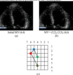
The final best motion velocity displacement point obtained in the predicted ventricular ultrasound image in Figure 5(b) is coordinated at (3, 1). The output produced in Figure 5 is considered as vector displacement smoothing. This is because the PSNR points have been improved for the same image sequence. At the same time the processing time is reduced after the Gaussian Filter is applied to suppress the high level of noise in the ultrasound image sequence.

Illustration in Figure 5(c) shows the motion velocity translations analysis compared to motion velocity translations analysis in Figure 4(c). The motion velocity translations analysis illustration in Figure 5(c) shows the motion translation after suppressing the ventricular ultrasound image sequence using the Gaussian Filter. After the noise suppression in the noisy ultrasound images, the motion moves away from the reference point.

According to the motion velocity in Figure 4(c), observation shows the motions magnitude subsists in increasing order. This explains that the motion velocity displacement point is moving inconstantly away from the reference point. The tru e best matching motion in Figure 3(b) is positioned at the vertical plane.

The motion velocity magnitudes in Figure 5(c) are in increasing order towards the vertical plane. According to the motion velocity displacement point in Figure 5(c) the final best matching displacement point is positioned at the vertical plane. While referring to the Table II and Table IV, the PSNR points have improved when the Gaussian Filter is applied to the ultrasound image sequences. This shows that, the PSNR points can be improved with suppressing the high level of noise in the ultrasound image sequences. At the same time, the processing time can be reduced.

V. CONCLUSION

In this studied, we present the HDDP algorithm which is appropriate to search the motion velocity displacement point. The HDDP algorithm is designed to optimize the block-matching technique for motion velocity in ultrasound image sequences. Such motion velocity displacement point is useful as a diagnostic tool. The result shows that the motion velocity displacement technique can be conducted as a diagnostic tool for examination purposes.

Initial MV (4,4) MV = (5,2), (4,1), (3,1)

(a) (b)

(c)

Fig. 5. (a) Original ultrasound image (b) Predicted ultrasound image with Gaussian Filter (c) Motion Velocity displacement point with Gaussian

Filter

TABLE III

SIMULAT ION RESULT AT 5 FRAMES WIT HOUT GAUSSIAN FILT ER

Original HDS

TABLE IV

SIMULAT ION RESULT AT 5 FRAMES WIT H GAUSSIAN FILT ER

HDS + Gaussian Filter

Initial MV (4,4) MV = (5,2), (5,6), (4,7)

(a) (b)

(c)

4

6 2 1

3

5

7 7 6 5 4 3 2 1

4

6 2 1

3

5

(5)

Fig. 6.(a) Original cardiovascular ultrasound image (b) Predicted cardiovascular ultrasound image (c) Motion Velocity displacement point.

Figure 6 shows the result for cardiovascular ultrasound image sequences. This image sequences is conducted without using the Gaussian Filter. The motion velocity displacement point obtained in the predicted cardiovascular ultrasound image in Figure 6(b) is coordinated at (4, 7). This image sequences is conducted to test the algorithm simulation on various type of image sequences.

According to the motion velocity in Figure 6(c), observation shows the motions magnitude subsists in increasing order. This explains that the motion velocity displacement point is moving inconstantly away from the reference point. The true best matching motion in Figure 6(b) is positioned at the vertical plane.

The result in Figure 7 is obtained using the Gaussian Filter. Based on the results, Figure 6(b) is the predicted cardiovascular ultrasound image. The final best motion velocity displacement point obtained in the predicted cardiovascular ultrasound image in Figure 6(c) is coordinated at (4, 6).

The motion velocity magnitudes in Figure 7(c) are in decreasing order towards the horizontal plane. The best matching displacement point in Figure 7(c) is decreasing towards the reference point. According to the motion velocity displacement point in Figure 7(c) the final best matching displacement point is positioned at the vertical plane.

Initial MV (4,4) MV = (5,2), (5,3), (4,6)

(a) (b)

(c)

Fig. 7. (a) Original cardiovascular ultrasound image (b) Predicted cardiovascular ultrasound image with Gaussian Filter (c) Motion Velocity

displacement point with Gaussian Filter

REFERENCES

[1] L. Gao, K. J. Parker, R. M. Lerner, and S. F. Levinson, Imaging of the elastic properties of tissue—a review. Ultrasound Medical Biology, 22(8): 1996, pp. 959–977.

[2] I. A. Hein, and JrW. D. O’Brien, Current time–domain methods for assessing tissue motion by analysis from reflected ultrasound echoes—a review. IEEE Transactions Ultrasonic Ferroelectr Frequency Control, 40(2): 1993 pp. 84–102.

[3] G. E. Mailloux, F. Langlois, P. Y. Simard, and M. Bertrand, Restoration of t he velocity field of the heart from two-dimensional echocardiograms. IEEE Transactions Medical Im aging, 8(2): 1989, pp.143–53.

[4] T .Georges, Smoothing the displacement field for edge-based motion estimation. Signal Processing V: Theories and Applications: 1990, pp. 967 – 970.

[5] J. L. Barron, D. J. Fleet, and S. S. Beauchemin, Performance of optical flow techniques. International Journal of Com puter Vision, 12: 1994, pp.43–77.

[6] J. Weber, and J. Malik, Robust computation of optical flow in a multi-scale differential framework. International Journal of Com puter Vision, 14(1): 1995, pp.67–81.

[7] S. A. Lai, and B. C. Vemuri, Robust and efficient computation of optical flow. International Journal of Com puter Vision, 29(2): 1998, pp.87–105.

[8] M. J. LedesmaCarbayo, J. Kybic, M. Sihling, P. Hunziker, M. Desco, A. Santos, and M. Unser, Cardiac ultrasound motion detection by elastic registration exploiting temporal coherence. In Proceedings IEEE International Sym posium on Biom edical Im aging: Washington DC, USA, 2002, pp. 585 –588.

[9] C. P. Bernard, Discrete wavelet analysis for fast optic flow computation. Internal Report RI415, France, 1999.

[10]S. Loncaric, and Z. Majcenic, Optical flow algorithm for cardiac motion estimation. Proceesing of the 22nd Annual International Conference of the Engineering in Medicine and Biology Society: 2000, pp. 415-417.

[11]Y. Huang, K. Palaniappan, X. Zhuang, and J.E. Cavanough, Optic flow field segmentation and motion estimation using a robustgenetic partitioning algorithm. IEEE Transactions on Pattern Analysis and Machine Intelligence:1995, pp. 1177 – 1190. [12]C. Kontogeorgakis, M. G. Strintzis, N. Maglaveras, and I.

Kokkinidis, T umor detection in ultrasound B-mode image through estimation using a texture detection algorithm, Proceedings 1994 Com puter Cardiology Conference, 1994, pp. 117–120.

[13]F. Yeung, S. F. Levinson, and K. J. Parker, Multilevel and motion model-based ultrasonic speckle tracking algorithms, Ultrasound Medical Biology, 24(3): 1998, pp. 427–441.

[14]V. Behar, D. Adam, P. Lysyansky, and Z. Friedman, Improving motion estimation by accounting for local image distortion. Journal of the Am erica Society of Echocardiography, 20: 2004, pp. 165-170.

[15]M. G. Linguraru, A. Kabla, N. V. Vasilyev, P. J. del Nido, and R. D. Howe, Real-time Block Flow T racking of Atrial Septal Defect Motion in 4D Cardiac Ultrasound. Biom edical Im aging, 2007, pp. 356 – 359.

[16]M. Shizawa, and K. Mase, Simultaneous multiple optical flow estimation. IEEE Conference Com puter Vision and Pattern Recognition, 1990, 274–278.

[17]D. Vernon, Decoupling Fourier components of dynamic image sequences: a theory of signal separation, image segmentation and optical flow estimation. Proceedings Europe Conference Computer Vision ECCV’98, 1998, pp. 68–85.

[18]Djamal Boukerroui, Alison Noble J., and Micheal Brady., Velocity estimation in Ultrasound Images: A Block Matching Approach. Lecture Notes in Com puter Science, 2003, pp. 586–598.

4

6 2 1

3

5