Image Mining for Mammogram Classification to detect breast cancer by Association Reverse Rule Using Statistical and GLCM features

Volume 5 Issue 2– June 2016 1 ISSN : 2319-6319

Image Mining for Mammogram Classification

to detect breast cancer by Association Reverse

Rule Using Statistical and GLCM features

Aswini Kumar Mohanty

Bhubaneswar, Orissa, India

Amalendu Bag

Department Of Computer Science, KMBB College of engg & CET Bhubaneswar – 752 054, Orissa, India

Abstract - The image mining technique deals with the extraction of implicit knowledge and image with data relationship or other patterns not explicitly stored in the images. It is an extension of data mining to image domain. The main objective of this paper is to apply image mining in the domain such as breast mammograms to classify and detect the cancerous tissue. Mammogram image can be classified into normal, benign and malignant class and to explore the feasibility of data mining approach. Results will show that there is promise in image mining based on content. It is well known that data mining techniques are more suitable to larger databases than the one used for these preliminary tests. In particular, a Computer aided method based on association rules becomes more accurate with a larger dataset. Traditional association rule algorithms adopt an iterative method to discovery frequent item set, which requires very large calculations and a complicated transaction process. Because of this, a new association rule algorithm is proposed in this paper. Experimental results show that this new method can quickly discover frequent item sets and effectively mine potential association rules. A total of 26 features including histogram intensity features and GLCM features are extracted from mammogram images. Experiments have been taken for a data set of 322 images taken from MIAS of different types with the aim of improving the accuracy by generating minimum no. of rules to cover more patterns. The accuracy obtained by this method is approximately 97% which is highly encouraging.

Keywords: Mammogram, Gray Level Co-occurrence Matrix feature, Histogram Intensity, Contrast Limited Adaptive Histogram Equalization Association rule mining, Reverse Rule Generation algorithm.

I. I.NTRODUCTION

Breast Cancer is one of the most common cancers, leading to cause of death among women, especially in developed countries. There is no primary prevention since cause is still not understood. So, early detection of the stage of cancer allows treatment which could lead to high survival rate. Mammography is currently the most effective imaging modality for breast cancer screening. However, 10-30% of breast cancers are missed at mammography [1]. Mining information and knowledge from large database has been recognized by many researchers as a key research topic in database system and machine learning Researches that use data mining approach in image learning can be found in [2,3].

Data mining of medical images is used to collect effective models, relations, rules, abnormalities and patterns from large volume of data. This procedure can accelerate the diagnosis process and decision-making. Different methods of data mining have been used to detect and classify anomalies in mammogram images such as wavelets [4,5], statistical methods and most of them used feature extracted using image processing techniques [6].Some other methods are based on fuzzy theory [7,8] and neural networks [9]. In this paper we have used classification method called Decision tree classifier for image classification [10-12].

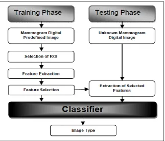
testing phase , these feature space partitions are used to classify the image. A block diagram of the method is shown in figure1.

Figure. 1.: Block diagram for mammogram classification system

We have used association rule mining using image content method by extracting low level image features for classification. The merits of this method are effective feature extraction, selection and efficient classification. The rest of the paper is organized as follows. Section 2 presents the preprocessing and section 3 presents the feature extraction phase. Section 4 discusses the proposed method of Feature selection and classification. In section5 the results are discussed and conclusion is presented in section 6.

II. II.METHODOLOGIES

2.1 Digital mammogram database

The mammogram images used in this experiment are taken from the mini mammography database of MIAS (http://peipa.essex.ac.uk/ipa/pix/mias/). In this database, the original MIAS database are digitized at 50 micron pixel edge and has been reduced to 200 micron pixel edge and clipped or padded so that every image is 1024 X 1024 pixels. All images are held as 8-bit gray level scale images with 256 different gray levels (0-255) and physically in portable gray map (pgm) format. This study solely concerns the detection of masses in mammograms and, therefore, a total of 100 mammograms comprising normal, malignant and benign case were considered. Ground truth of location and size of masses is available inside the database.

2.2 Pre-processing

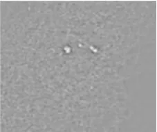
The mammogram image for this study is taken from Mammography Image Analysis Society (MIAS)†, which is an UK research group organization related to the Breast cancer investigation [13]. As mammograms are difficult to interpret, preprocessing is necessary to improve the quality of image and make the feature extraction phase as an easier and reliable one. The calcification cluster/tumor is surrounded by breast tissue that masks the calcifications preventing accurate detection and shown in Figure.2.(a). .A pre-processing; usually noise-reducing step [14] is applied to improve image and calcification contrast figure 2.(b). In this work the efficient filter (CLAHE) was applied to the image that maintained calcifications while suppressing unimportant image features. Figure 2.(c) shows representative output image of the filter for a image cluster in figure 2. By comparing the two images, we observe background mammography structures are removed while calcifications are preserved. This simplifies the further tumor detection step.

.Contrast limited adaptive histogram equalization (CLAHE) method seeks to reduce the noise produced in homogeneous areas and was originally developed for medical imaging [15]. This method has been used for enhancement to remove the noise in the pre-processing of digital mammogram [16]. CLAHE operates on small regions in the image called tiles rather than the entire image. Each tile’s contrast is enhanced, so that the histogram of the output region approximately matches the uniform distribution or Rayleigh distribution or exponential distribution. Distribution is the desired histogram shape for the image tiles. The neighboring tiles are then combined using bilinear interpolation to eliminate artificially induced boundaries. The contrast, especially in homogeneous areas, can be limited to avoid amplifying any noise that might be present in the image. The block diagram of pre-processing is shown in Figure 2©

Figure 2.(a). ROI of a Benign Figure 2.(b) ROI after Pre-processing Operation

Figure2.(c). Image pre-processing block diagram. 2.3 Histogram equalization

† peipa.essex.ac.uk/info/mias.html

III.FEATUREEXTRACTION

Features, characteristics of the objects of interest, if selected carefully are representative of the maximum relevant information that the image has to offer for a complete characterization a lesion [18, 19]. Feature extraction methodologies analyze objects and images to extract the most prominent features that are representative of the various classes of objects. Features are used as inputs to classifiers that assign them to the class that they represent. In this Work intensity histogram features and Gray Level Co-Occurrence Matrix (GLCM) features are extracted.

3.1Intensity histogram features

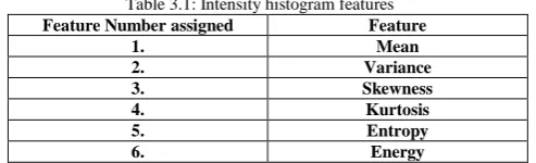
Intensity Histogram analysis has been extensively researched in the initial stages of development of this algorithm [18, 20]. Prior studies have yielded the intensity histogram features like mean, variance, entropy etc. These are summarized in Table 3.1 Mean values characterize individual calcifications; Standard Deviations (SD) characterize the cluster. Table 3.2 summarizes the values for those features.

Table 3.1: Intensity histogram features

Feature Number assigned Feature

1. Mean

2. Variance

3. Skewness

4. Kurtosis

5. Entropy

6. Energy

In this paper, the value obtained from our work for different type of image is given as follows: Table 3.2: Intensity histogram features and their values

Image Type

Features

Mean Variance Skewness Kurtosis Entropy Energy

normal 7.2534 1.6909 -1.4745 7.8097 0.2504 1.5152

malignant 6.8175 4.0981 -1.3672 4.7321 0.1904 1.5555

benign 5.6279 3.1830 -1.4769 4.9638 0.2682 1.5690

3.2 Glcm features

It is a statistical method that considers the spatial relationship of pixels is the gray-level co-occurrence matrix (GLCM), also known as the gray-level spatial dependence matrix [21, 22]. By default, the spatial relationship is defined as the pixel of interest and the pixel to its immediate right (horizontally adjacent), but you can specify other spatial relationships between the two pixels. Each element (I, J) in the resultant GLCM is simply the sum of the number of times that the pixel with value I occurred in the specified spatial relationship to a pixel with value J in the input image.

3.3 Glcm construction

An entry in the matrix S gives the number of times that gray level i is oriented with respect to gray level j such that W(x1, y1)=i and W(x2, y2)=j, then

We use two different distances d={1, 2} and three different angles θ={0°, 45°, 90°}. Here, angle representation is taken in clock wise direction.

Example

Intensity matrix

and

The Following GLCM features were extracted in our research work:

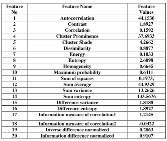
Autocorrelation, Contrast, Correlation, Cluster Prominence, Cluster Shade, Dissimilarity Energy, Entropy, Homogeneity, Maximum probability, Sum of squares, Sum average, Sum variance, Sum entropy, Difference variance, Difference entropy, information measure of correlation1, information measure of correlation2, Inverse difference normalized. Information difference normalized. The value obtained for the above features from our work for a typical image is given in the following table 3.3.

Table 3.3 : GLCM Features and values Extracted from Mammogram Image(Malignant)

Feature No

Feature Name Feature

Values

1 Autocorrelation 44.1530

2 Contrast 1.8927

3 Correlation 0.1592

4 Cluster Prominence 37.6933

5 Cluster Shade 4.2662

6 Dissimilarity 0.8877

7 Energy 0.1033

8 Entropy 2.6098

9 Homogeneity 0.6645

10 Maximum probability 0.6411

11 Sum of squares 0.1973,

12 Sum average 44.9329

13 Sum variance 13.2626

14 Sum entropy 133.5676

15 Difference variance 1.8188

16 Difference entropy 1.8927

17 Information measure of correlation1 1.2145

18 Information measure of correlation2 -0.0322

19 Inverse difference normalized 0.2863

IV.CLASSIFICATION 4.1 RRG algorithm

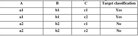
Reverse Rule Generation (RRG) algorithm generates association rules in a completely reverse way from the existing algorithms. Before describing the algorithm in formal definition, let’s take a look what we are going to do by an example. Say, we have the following training examples in table 4.1

Table 4.1: Transaction database for example of RRG algorithm:

A B C Target classification

a1 b1 c1 Yes

a1 b1 c2 Yes

a2 b2 c1 No

a2 b2 c2 No

At first we will fix a satisfactory Confidence. Say it is 50%. Then we will generate one rule from each training example. So, at first step we have 4 rules. They are like these:

R1: A=a1,B=b1,C=c1=>yes R2: A=a1,B=b1,C=c2=>yes R3: A=a2,B=b2,C=c1=>no R4: A=a2,B=b2,C=c2=>no

Note that all 4 rules have confidence 100%. These rules are enqueued in a queue (say it is q). Now dequeue a rule from q and remove one attribute constraint at a time. If R1 is dequeued then the 3 rules will be constructed by removing one attribute constraint at a time:

R11: A=a1,B=b1=>yes R12: B=b1,C=c1=>yes R13: A=a1,C=c1=>yes

Now enqueue the newly constructed rules in q that have confidence greater than or equal to satisfactory Confidence and go on in this way.

So, the RRG algorithm looks like this: 1. satisfactoryConfidence = 0.5;

2. ruleList = Φ 3. q= Φ

4. for each record rec training example 5. r = constructRule(rec);

6. ruleList = ruleList ∪ r; 7. enqueue(q,r);

8.while (q is not empty) 9. r = dequeue(q);

10. for each attribute A ∈ r 11. r2 = constructRule2(A, r);

13. ruleList = ruleList ∪ r2; 14. enqueue(q,r2);

Satisfactory Confidence and q are described earlier. Rule List is a list that will contain the generated CARs. Line 1-3 represents initialization. Line 4-7 describes how training examples having confidence greater than or equal to satisfactoryConfidence are directly converted to CARs. Construct Rule function (line 5) serves this purpose in a way described earlier. enqueue function enqueues rule r into queue q. Line 8-14 generates rules by removing one attribute at a time from the rules found by dequeuing q. constructRule2 function (line 11) is doing a major task by constructing rule r2 from r by removing attribute A. constructRule2 function also calculates the confidence of rule r2. Finally, we get all of our generated rules in ruleList.

4.2. Classifier construction

ruleList still contains a lot of rules. They all will not be used in the classifier. The classifier construction algorithm looks like this:

1. finalRuleSet = Φ dataSet = D; 2. sort(ruleList);

3. for each rule r ∈ ruleList

4. if r correctly classifies at least one training example d ∈ dataset then 5. remove d from dataset;

6. insert r at the end of finalRuleSet;

Lines 1-2 are for initialization purpose. finalRuleSet is a list that will contain rules that will be used in the classifier. sort function (line 3) sorts ruleList in descending order of confidence, support and rule length. Lines 4-6 take only those rules in the finalRuleSet which can correctly classify at least one traing example. Note that the insertion in finalRuleSet ensures that all the rules of finalRuleSet will be sorted in descending order of confidence, support and rule length.

When a new test example is to be classified, classify according to the first rule in the finalRuleSet that covers the test example.

There is no support pruning. All associative classification algorithms use a very low support threshold (as low as 1%) to generate association rules. In that way some high quality rules that have higher confidence, but lower threshold will be missed. Here we are getting those high quality rules as there is no support pruning.

V.EXPERIMENTALRESULTS

Learning package, WEKA [27]. Out of 322 images in the dataset, 208 were used for training and the remaining 114 for testing purposes.

Table 5.1: Results obtained by proposed method

Normal 100%

Malignant 88. 23%

Benign 97.11%

The confusion matrix has been obtained from the testing part. In this case for example out of 51 actual malignant images 06 images was classified as normal. In case of benign all images are correctly classified and in case of normal images 6 images are classified as malignant. The confusion matrix is given in Table 5.2.

Table 5.2: Confusion matrix

Actual Predicted class

Benign Malignant Normal

Benign 63 0 0

Malignant 51 45 06

Normal 208 6 202

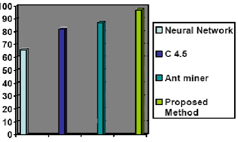
The following graph shows the comparative analysis of our method and various other methods.

Figure. 5. Performance of the Classifier

VI.CONCLUSION

fact it can be proved that RRG generates the complete set of high confidence rules.

Although by now some progress has been achieved, there are still remaining challenges and directions for future research, such as, developing better preprocessing, enhancement and segmentation techniques; designing better feature extraction, selection and classification algorithms; integration of classifiers to reduce both false positives and false negatives; employing high resolution mammograms and investigating 3D mammograms. The CAD mammography systems for micro calcifications detection have gone from crude tools in the research laboratory to commercial systems. Mammogram image analysis society database is standard test set but defining different standard test set (database) and better evaluation criteria are still very important. With some rigorous evaluations, and objective and fair comparison could determine the relative merit of competing algorithms and facilitate the development of better and robust systems. The methods like one presented in this paper could assist the medical staff and improve the accuracy of detection. Our method can reduce the computation cost of mammogram image analysis and can be applied to other image analysis applications. The algorithm uses simple statistical techniques in collaboration to develop a novel feature selection technique for medical image analysis. The value of this technique is that it not only tackles the measurement problem but also provides a visualization of the relation among features. In addition to ease of use, this approach effectively addresses the feature redundancy problem. The method proposed has been proven that it is easier and it requires less computing time than existing methods.

REFERENCES

[1] Majid AS, de Paredes ES, Doherty RD, Sharma N Salvador X. “Missed breast carcinoma: pitfalls and Pearls”.Radiographics, pp.881-895, 2003.

[2] Osmar R. Zaïane,M-L. Antonie, A. Coman “Mammography Classification by Association Rule based Classifier,” MDM/KDD2002 International Workshop on Multimedia Data Mining ACM SIGKDD, pp.62-69, 2002,

[3] Xie Xuanyang, Gong Yuchang, Wan Shouhong, Li Xi ,”Computer Aided Detection ofSARS Based on Radiographs Data Mining “, Proceedings of the 2005 IEEE Engineering in Medicine and Biology 27th Annual Conference Shanghai, China, pp7459 – 7462, 2005. [4] C.Chen and G.Lee, “Image segmentation using multitiresolution wavelet analysis and Expectation Maximum(EM) algorithm for

mammography” , International Journal of Imaging System and Technology, 8(5): pp491-504,1997

[5] T.Wang and N.Karayaiannis, “Detection of microcalcification in digital mammograms using wavelets”, IEEE Trans. Medical Imaging, 17(4):498-509, 1998.

[6] Jelena Bozek, Mario Mustra, Kresimir Delac, and Mislav Grgic “A Survey of Image Processing Algorithms in Digital mammography”Grgic et al. (Eds.): Rec. Advan. in Mult. Sig. Process. and Commun., SCI 231, pp. 631–657,2009

[7] Shuyan Wang, Mingquan Zhou and Guohua Geng, “Application of Fuzzy Cluster analysis for Medical Image Data Mining” Proceedings of the IEEE International Conference on Mechatronics & Automation Niagara Falls, Canada,pp. 36 – 41,July 2005. [8] R.Jensen, Qiang Shen, “Semantics Preserving Dimensionality Reduction: Rough and Fuzzy-Rough Based Approaches”, IEEE

Transactions on Knowledge and Data Engineering, pp. 1457-1471, 2004.

[9] I.Christiyanni et al ., “Fast detection of masses in computer aided mammography”, IEEE Signal processing Magazine, pp:54- 64,2000 [10] Walid Erray, and Hakim Hacid, “A New Cost Sensitive Decision Tree Method Application for Mammograms Classification” IJCSNS

International Journal of Computer Science and Network Security, pp. 130-138, 2006.

[11] Ying Liu, Dengsheng Zhang, Guojun Lu, Regionbased “image retrieval with high-level semantics using decision tree learning”, Pattern Recognition, 41, pp. 2554 – 2570, 2008.

[12] Kemal Polat , Salih Gu¨nes, “A novel hybrid intelligent method based on C4.5 decision tree classifier and one-against-all approach for multi-class classification problems”, Expert Systems with Applications, Volume 36 Issue 2, pp.1587-1592, March, 2009, doi:10.1016/j.eswa.2007.11.051

[13] Etta D. Pisano, Elodia B. Cole Bradley, M. Hemminger, Martin J. Yaffe, Stephen R. Aylward, Andrew D. A. Maidment, R. Eugene Johnston, Mark B. Williams,Loren T. Niklason, Emily F. Conant, Laurie L. Fajardo,Daniel B. Kopans, Marylee E. Brown • Stephen M. Pizer “Image Processing Algorithms for Digital Mammography: A Pictorial Essay” journal of Radio Graphics Volume 20,Number 5,sept.2000

[14] Pisano ED, Gatsonis C, Hendrick E et al. “Diagnostic performance of digital versus film mammography for breast-cancer screening”. NEngl J Med 2005; 353(17):1773-83.

[15] Wanga X, Wong BS, Guan TC. ‘Image enhancement for radiography inspection”. International Conference on Experimental Mechanics. 2004: 462-8.

[17] Dougherty J, Kohavi R, Sahami M. “Supervised and unsupervised discretization of continuous features”. In: Proceedings of the 12th international conference on machine learning.San Francisco:Morgan Kaufmann; pp 194–202, 1995.

[18] Yvan Saeys, Thomas Abeel, Yves Van de Peer “Towards robust feature selection techniques”, www.bioinformatics.psb.ugent [19] Gianluca Bontempi, Benjamin Haibe-Kains “Feature selection methods for mining bioinformatics data”, http://www.ulb.ac.be/di/mlg [20] Li Liu, Jian Wang and Kai He “Breast density classification using histogram moments of multiple resolution mammograms”

Biomedical Engineering and Informatics (BMEI), 3rd International Conference, IEEE explore pp.146–149, DOI: November 2010, 10.1109/ BMEI.2010 .5639662,

[21] Li Ke,Nannan Mu,Yan Kang Mass computer-aided diagnosis method in mammogram based on texture features, Biomedical Engineering and Informatics (BMEI), 3rd International Conference, IEEE Explore, pp.146 – 149, November 2010, DOI: 10.1109/ BMEI.2010.5639662,

[22] Azlindawaty Mohd Khuzi, R. Besar and W. M. D. Wan Zaki “Texture Features Selection for Masses Detection In Digital Mammogram” 4th Kuala Lumpur International Conference on Biomedical Engineering 2008 IFMBE Proceedings, 2008, Volume 21, Part 3, Part 8, 629-632, DOI: 10.1007/978-3-540-69139-6_157

[23] S.Lai,X.Li and W.Bischof “On techniques for detecting circumscribed masses in mammograms”, IEEE Trans on Medical Imaging , 8(4): pp. 377-386,1989.

[24] Somol, P.Novovicova, J..Grim, J., Pudil, P.” Dynamic Oscillating Search Algorithm for Feature Selection” 19th International

Conference onPattern Recognition, 2008. ICPR 2008. pp.1-4 D.O.I10.1109/ICPR.2008.4761773

[25] R. Kohavi and G. H. John. “Wrappers for feature subset selection”. Artif. Intell., 97(1-2):273–324, 1997.

[26] Deepa S. Deshpande “ASSOCIATION RULE MINING BASED ON IMAGE CONTENT” International Journal of Information Technology and Knowledge Management January-June 2011, Volume 4, No. 1, pp. 143-146

[27] Holmes, G., Donkin, A., Witten, I.H.: WEKA: a machine learning workbench. In Proceedings Second Australia and New Zealand Conference on Intelligent Information Systems, Brisbane, Australia, pp. 357-361, 1994.