Performance and Complexity Comparison of Channel Estimation Algorithms for OFDM System

Performance and Complexity Comparison of

Channel Estimation Algorithms for OFDM

System

Saqib Saleem

1

_{, Qamar-Ul-Islam}

2

Department of Communication System Engineering, Institute of Space Technology Islamabad, Pakistan

1_{[email protected],} 2_{[email protected]}

Abstract-- To mitigate the multipath delay effect of the received signal, the information of the time-varying channel is required at the receiver to determine the equalizer co-efficients. In this paper two basic algorithms, known as Linear Minimum Mean Square (LMMSE) and Least Square Error (LSE), are discussed which make use of the channel statistics in time domain. To reduce the complexity, different variants of these algorithms are also discussed. Channel Impulse Response (CIR) samples and channel taps are used to compare the performance and complexity. MATLAB simulations are carried out to compare the performance in terms of Mean Square Error (MSE) and Symbol Error Rate (SER) of these algorithms for different modulation techniques.

Index Term-- Mean Square Error, Channel Impulse Response, Least Square Error, Minimum Mean Square Error, Channel Taps.

I.

INTRODUCTION

For high data rate communication systems like next generation (4G) wireless networks, operated in frequency selective fading environments, a multi carrier modulation technique is used, commonly known as Orthogonal Frequency Division Multiplexing (OFDM). This technique is used for extenuating the Inter-symbol Interference (ISI) to enhance the channel’s capability using spectral efficiency. Quality of service can also be improved, when we merge OFDM technique with Multiple-Input Multiple-Output (MIMO) in which there is no need to assign additional bandwidth to channel.

MIMO systems that use coherent OFDM can provide high channel capability if there is precise information of the channel available at the receiver. This performance can even be increased if the Channel State Information (CSI) is also available at the transmitter because it makes our receiver design simpler [1]. The performance of the system usually relies on the channel estimation algorithm. Decision directed channel estimation and pilot- assisted channel estimation are the two basic methods for channel estimation. In decision directed method, there is no need of additional pilots because recovered data is treated as “new pilots” that provides the

channel estimation module with that data which keeps track of the state of channel and provides the advantage of less delay as compared to other techniques such as interpolation, Wiener or Kalman Filtering. However this method has some disadvantages like its response to error detection is not suitable that causes error propagation and the need of huge amount of data slow down its convergence rate. In pilot-assisted method we collect channel information from the pilots that are transmitted with the signal using interpolation filters. There are two modes of pilot-assisted channel estimation method, one in which all subcarriers are used aspilots for a specific period known as block pilot mode and the other one is comb pilot mode in which some of the subcarriers are used as pilots.

Two basic algorithms can be considered for channel estimation using pilot-assisted technique. First one is Least Square Estimation (LSE) and the other one is Linear MinimumMean Square Estimation (LMMSE). LSE has less complexity as there is no need of any channel apriority probability that’s why it is easy to implement, but to attain superior performance LMMSE is preferred which is based on channel autocorrelation matrix in frequency domain. It minimizes the Mean Square Error (MSE) of the channel by utilizing the information of operating SNR and the channel statistics due to which its complexity is higher [2]. To overcome this problem a low-rank approximation to LMMSE has been proposed by using singular value decomposition (SVD) [3].Complexity of this algorithm can also be reduced by the use of channel taps and Channel Impulse response (CIR) samples. To achieve better results in channel estimation we have to keep track of some further parameters like channel statistics, the channel Power Delay Profile (PDP) available to the receiver and assistance of decoder feedbacks.

In Section II, signal and channel model is discussed and Section III describes the theoretical analysis of channel estimation algorithms. Section IV shows the simulation results and conclusions are drawn in last section.

the sampling period will be T/N. If 𝐷𝑖,𝑛 is data on the nth sub-carrier in the ith _{OFDM symbol then the transmitted symbol} will be [4]

𝑠(𝑡) = ∑ ∑𝑁−1𝐷𝑖,𝑛𝜃𝑖,𝑛(𝑡) 𝑛=0

∞

𝑖=−∞ (1)

Where 𝜃𝑖,𝑛(𝑡) is given by

𝜃𝑖,𝑛(𝑡) = 𝑒𝑗2𝜋𝑛𝑇 (𝑡−𝑇𝑔−𝑖𝑇𝑐)

[𝑢(𝑡 − 𝑖𝑇𝑐) − 𝑢(𝑡 − (𝑖 + 1)𝑇𝑐)] (2)

𝑇𝑔 is guard time interval, inserted to avoid interference. 𝑇𝑐 = 𝑇𝑔+ 𝑇 is total symbol duration. In this case the signal passed through a multipath channel characterized by

𝑔(𝑡, 𝜏) = ∑𝐿−1𝑖=0𝛼𝑖𝛿(𝑡 − 𝜏𝑖) (3)

Where 𝛼𝑖 is the time-varying gain having complex Rayleigh Distribution 𝜏𝑖 is time-delay for the ith _{multipath and L is total} number of multipaths. After passing through fast fading multipath channel the received signal will be

𝑟(𝑡) = ∑𝐿−1𝛼𝑖𝛿(𝑡 − 𝜏𝑖)

𝑖=0 + 𝑛(𝑡) (4)

In frequency domain the received signal on the kth _sub-carrier of the sth _{symbol is}

𝑌𝑠,𝑘= 𝐷𝑠,𝑘. 𝐻𝑠,𝑘+ 𝑁𝑠,𝑘 (5)

Where 𝐻 is the channel frequency response, which is the DFT of the channel impulse response vector 𝑔(𝑡, 𝜏).

III.

CHANNEL ESTIMATION ALGORITHMS

A. LMMSE Channel Estimation

After passing through AWGN channel having the noise variance 𝜎𝑛2_{, the LMMSE estimation of the channel} vector 𝑔 is given by [5]

𝑔̂ = 𝚪𝑔𝑦𝚪𝑦𝑦−1𝑦 (6) Where

𝚪𝑔𝑦 = 𝚪𝑔𝑔𝐹𝐻𝑋𝐻

𝚪𝑦𝑦 = 𝑋𝐹𝚪𝑔𝑔𝐹𝐻_𝑋𝐻_{+ 𝜎} 𝑛2𝐼𝑁

Where𝚪𝑔𝑦 is the cross co-variance matrix between 𝑔 and 𝑦 and 𝚪𝑦𝑦 is the auto-covariance matrix of 𝑦. These co-variance matrices should be positive definite to make a unique minimum MSE.

The channel estimate ℎ̂𝑚𝑚𝑠𝑒 , in frequency domain, is obtained by taking DFT of 𝑔̂, given by

ℎ̂𝑚𝑚𝑠𝑒= 𝐹𝑔̂ = 𝐹𝑄𝐹𝐻𝑋𝐻𝑦 (7)

Where 𝐹 is orthonormal DFT-matrix and 𝑄 is given by [4] 𝑄 = 𝚪𝑔𝑔[(𝐹𝐻𝑋𝐻𝑋𝐹)−1𝜎𝑛2+ 𝚪𝑔𝑔]

−1

(𝐹𝐻_𝑋𝐻_𝑋𝐹)−1 (8)

B. Low Complex LMMSE Channel Estimation

Inversion of a large matrix is required in LMMSE channel estimation. The complexity of LMMSE increases especially when the input data 𝑋 changes and the matrix inversion is needed recursively. If same modulation constellation is considered for each OFDM symbol, then the average of the input data 𝑋 becomes

𝐸(𝑋𝑋𝐻₎−1_{= 𝐸 |}1 𝑥𝑘 |

2 .

And low complex LMMSE estimation is given by [6] ℎ̂𝑚𝑚𝑠𝑒 = 𝚪𝑔𝑔(𝚪𝑔𝑔+

𝛽 𝑆𝑁𝑅𝐼)

−1_𝑋−1_{𝑦 (9)}

Where 𝛽 depends upon the constellation of the modulation technique used for OFDM symbol.

C. Modified LMMSE Channel Estimation

For large size input data X, the calculation of Q matrix increases the complexity of LMMSE estimation. If the taps having significant energy are considered only, then for L taps, 𝚪𝑔𝑔 becomes a L × L matrix and in this case the modified LMMSE becomes [5]

ℎ̂𝑚𝑚𝑠𝑒= 𝑇𝑄′𝑇𝐻𝑋𝐻𝑦 (10)

Where T is a matrix having only first L columns of DFT matrix F and for this reduced complexity case 𝑄′ is

𝑄′= 𝚪′𝑔𝑔[(𝑇𝐻_𝑋𝐻_𝑋𝑇)−1_𝜎

𝑛2+ 𝚪′𝑔𝑔] −1

(𝑇𝐻_𝑋𝐻_𝑋𝑇)−1 (11)

Where 𝚪′𝑔𝑔 is the upper left L ×L matrix of 𝚪𝑔𝑔.

D. Robust LMMSE Channel Estimation

The behavior of the channel also changes especially for high mobility wireless links due to the time-varying surrounding environment [7]. In such a situation, the channel PDP is difficult to know. If all PDP’s are assumed to be having same maximum delay then the channel co-variance matrix with a uniform PDP gives better performance [8].

E. LSE Channel Estimation

In real time situations, a prior knowledge about the channel and noise statistics is not possible, that is why we design a filter that is function of input data only. No probabilistic assumptions are required for LSE channel estimation [9].

LSE estimation of channel vector 𝑔 is given by ℎ̂𝑙𝑠= 𝐹𝑄𝑙𝑠𝐹𝐻𝑋𝐻𝑦 (12) where

𝑄𝑙𝑠= (𝐹𝐻𝑋𝐻𝑋𝐹)−1

ℎ̂𝑙𝑠 is also given by [4]

F. Modified LSE Channel Estimation

There is no doubt that LSE is less complex, but the consideration of only high energy channel taps can further improve the performance. The modified LSE estimator, taking into account only L taps, is given by

ℎ̂𝑙𝑠= 𝑇𝑄𝑙𝑠′ 𝑇𝐻𝑋𝐻𝑦 (14) where

𝑄𝑙𝑠′ = (𝑇𝐻𝑋𝐻𝑋𝑇)−1

G. Regularized LSE Channel Estimation

The inversion of a large matrix can be simplified by regularizing its Eigen values, for which a constant term is added to its diagonal elements. Now the matrix 𝑄𝑙𝑠 can be written as [10]

𝑄𝑟𝑒𝑔,𝑙𝑠= (𝛼𝐼 + 𝐹𝐻𝑋𝐻𝑋𝐹)−1 (15)

Where the value of offline constant 𝛼 is selected to make the matrix 𝑄𝑟𝑒𝑔,𝑙𝑠 least perturbed.

H. Down-Sampled Impulse Response LSE Channel Estimation

The complexity of inversion of a large matrix can also be reduced by decreasing the sampling frequency. Some channel taps can be discarded and remaining taps are used for channel estimation. If the down-sampling rate is 1/3, then the down-sampled channel vector 𝑔 becomes [2]

𝑔̅ = (𝑔0 𝑔1 0 𝑔3 𝑔4 0 … 𝑔𝐿−1)𝑻

The channel in frequency domain can be written as

𝐻𝐷𝑆_{= 𝐹𝑔̅} Which is equivalent to

𝐻𝐷𝑆

=

[

1 1 1 1 1

1 𝑤1 _𝑤3 _{… 𝑤}(𝐿−1)

1 𝑤2 𝑤6 … 𝑤2(𝐿−1)

1 𝑤3 _𝑤9 _{… 𝑤}3(𝐿−1)

1 𝑤4 _𝑤12 _{… 𝑤}4(𝐿−1)

1 𝑤5 _𝑤15 _{… 𝑤}5(𝐿−1)

1 … … … …

1 𝑤𝑁−1 _𝑤3(𝑁−1) _{… 𝑤}(𝑁−1)(𝐿−1)_] [

𝑔0 𝑔1 𝑔3 𝑔4 ⋮ 𝑔𝐿−1]

And the LSE estimated channel will be

ℎ̂𝐷𝑆= (𝐹𝐷𝑆,𝐻_𝑋𝐻_𝑋𝐹𝐷𝑆₎−1_𝐹𝐷𝑆,𝐻_𝑋𝐻_{𝑦 (16)}

IV. SIMULATION RESULTS

In this section MATLAB simulation results are presented and discussed. The performance and complexity of the proposed algorithms is evaluated in terms of Mean Square Error (MSE) and Symbol Error Rate (SER). In these simulations, the modulation schemes considered are BPSK, QPSK and 8-PSK. For an OFDM signal, 64-point FFT is employed and Jake’s

Model is simulated for Rayleigh fading channel. The effect of SNR value, channel impulse response (CIR) and channel taps in relation to performance and computational time is evaluated.

a) Comparison of LMMSE Channel Estimators

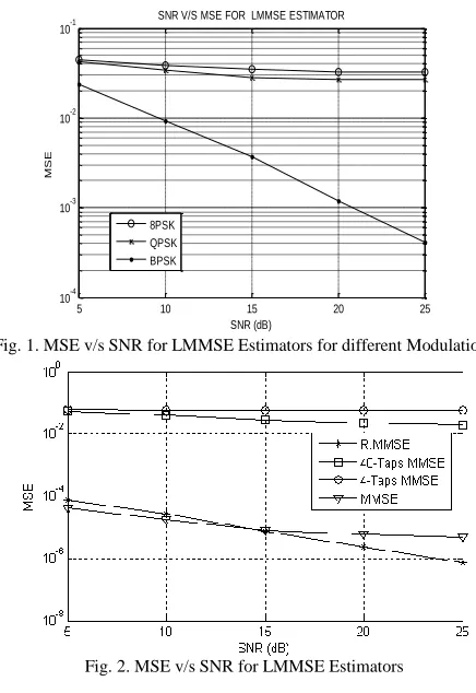
The performance of LMMSE Estimator for different modulation schemes is shown in Fig.1 as a function of SNR values. For BPSK, the performance is better that for QPSK and 8-PSK, but the later modulations result in high transmission rate. The comparison of LMMSE with modified LMMSE and Robust LMMSE is demonstrated in Fig.2. The performance degradation of modified LMMSE is due to the fact that some of the channel statistics are ignored. The R.LMMSE algorithm shows better performance behavior for higher SNR than LMMSE but for low SNR values, LMMSE is better choice. The complexity of Low complex LMMSE is less than LMMSE but the MSE behavior remains same.

Fig. 1. MSE v/s SNR for LMMSE Estimators for different Modulations

Fig. 2. MSE v/s SNR for LMMSE Estimators

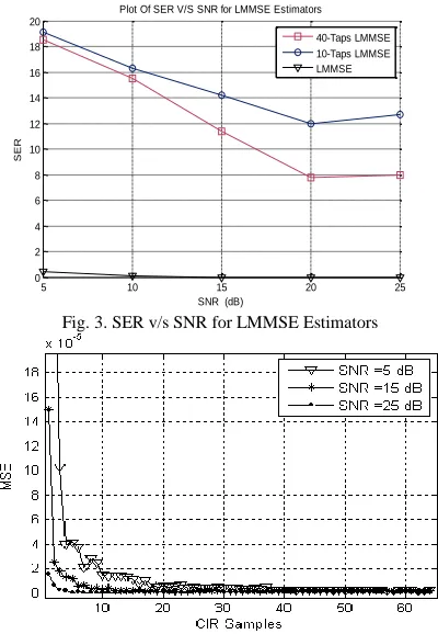
Fig.3 shows the performance of LMMSE estimators in terms of Symbol Error Rate (SER). The LMMSE outperforms the modified LMMSE algorithms because in later techniques, some of the channel statistics are ignored. The complexity of different LMMSE estimators is compared in Table 1.

5 10 15 20 25

10-4 10-3 10-2 10-1

SNR (dB)

M

S

E

SNR V/S MSE FOR LMMSE ESTIMATOR

Fig. 3. SER v/s SNR for LMMSE Estimators

Fig. 4. MSE v/s CIR Samples for LMMSE Estimator

Fig. 5. SER v/s Channel Taps for Modified LMMSE Estimator

The

effect of CIR Samples on performance of LMMSE estimators is shown in Fig.4. As number of CIR samples increases beyond a certain number, the effect of SNR value does not matter on the performance. However the complexity increases 50% as CIR samples increase from 30 to 50.

TABLE I

COMPUTATIONAL TIME FOR LMMSE ESTIMATORS

Estimator 5000 Simulations (sec)

1 OFDM Symbol (mSec)

1 Bit (mSec)

LMMSE Modified-10

208.278 41.656 0.651

Low Complex

LMMSE

320.713 64.143 1.003

LMMSE (Corr Mtx)

346.8 69.36 1.084

LMMSE Modified-40

440.945 88.189 1.378

R.LMMSE 528.133 105.627 1.651

LMMSE (Cov

Mtx)

529.319 105.864 1.65

The performance improves significantly as number of channel taps increases to 10, but after that there is no improvement in MSE. So increasing the channel taps after 10, only complexity increases such that as we go from 30 to 50 channel taps, the complexity increases 100%.

Fig.5 shows the performance in terms of SER, as a function of channel taps for different SNR values for modified LMMSE Estimators. The performance also remains same for channel taps from 10 to 60 and after 60 channel taps, the performance improves slightly.

b) Comparison of LSE Estimators

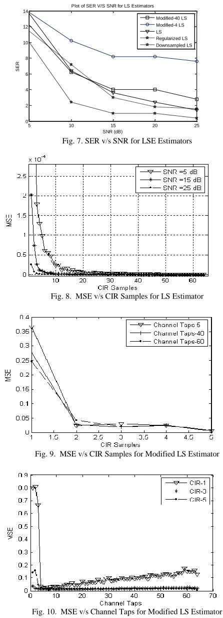
Fig.6 shows the performance comparison of different LSE algorithms in terms of MSE. For small SNR values, the modified LSE shows improved performance, but for higher SNR values, the behavior is same as that of modified LMMSE estimators. Regularized LSE estimator demonstrates a degraded performance at higher SNR values. Advantages of down-sampled LSE is only in terms form of less computational time. The performance remains same as that of LSE estimator. The performance in terms of SER for different SNR values is shown in Fig.7.

The effect of CIR samples on MSE of LSE estimator is shown in Fig.8. The performance improves significantly for CIR samples from 0 to 10, but then there is no improvement in performance and only complexity goes on increasing. The computational time for different CIR samples is shown in Table 2. The performance for different channel taps is shown in Fig.9, as a function of CIR samples and MSE. Beyond a specific value of

Fig. 6. MSE v/s SNR for LS Estimators

5 10 15 20 25

0 2 4 6 8 10 12 14 16 18 20

SNR (dB)

SER

Plot Of SER V/S SNR for LMMSE Estimators

40-Taps LMMSE 10-Taps LMMSE LMMSE

0 10 20 30 40 50 60 70

0 5 10 15 20 25 30 35 40

SER v/s Channel Taps for Modified LMMSE Estimator

Channel Taps

SER

Fig. 7. SER v/s SNR for LSE Estimators

Fig. 8. MSE v/s CIR Samples for LS Estimator

Fig. 9. MSE v/s CIR Samples for Modified LS Estimator

Fig. 10. MSE v/s Channel Taps for Modified LS Estimator

CIR samples, the MSE remains same irrespective of the channel taps. MSE, for different CIR samples, as a

function of channel taps is shown in Fig.10. MSE for different down-sampled LSE estimators is shown in Fig.11. The computational time decreases significantly while increasing the down-sampling rate, but at the cost of degraded performance.

Fig. 11. MSE v/s SNR for Down-Sampled LS Estimators

TABLE II

TIME V/S CIR SAMPLES FOR LS ESTIMATOR

CIR Samples Time (mSec)

30 0.5

40 1

50 1.25

60 1.5

c) Comparison of LSE and LMMSE Channel Estimators

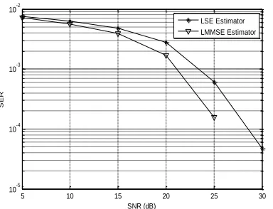
The performance of LSE and LMMSE estimator in terms of MSE as a function of SNR is compared in Fig.12. For less CIR samples, LMMSE outperforms LSE in terms of less MSE, not in terms of complexity. But by increasing CIR samples, LSE’s performance improves for higher SNR values and if we increase CIR samples further, then LSE starts to show better performance for all SNR values. The computational time of both LSE and LMMSE, for different CIR samples is compared in Table 3. SER performance comparison of LSE and LMMSE is shown in Fig. 13. The performance of LMMSE is better as it utilizes the channel statistics.

Fig. 12. MSE v/s SNR for LMMSE and LSE Estimators with different CIR Samples

5 10 15 20 25

0 2 4 6 8 10 12 14

SNR (dB)

SER

Plot of SER V/S SNR for LS Estimators

Fig. 13. SER v/s SNR for LSE and LMMSE Estimators

TABLE III

TIME V/S CIR SAMPLES FOR LMMSE AND LS ESTIMATOR

V. CONCLUSIONS

In this paper, the performance and complexity of two algorithms, LSE and LMMSE, is evaluated in terms of MSE and SER, based on CIR samples and channel taps. LMMSE is capable of improving the performance by making use of a prior information of noise and channel. But this improved performance comes at the cost of more complexity. The performance can be improved by increasing CIR samples or channel taps but after a certain value of these factors, only complexity increases and the performance does not have any further improvement. LSE can be made more efficient both in term of performance and complexity by increasing CIR samples than LMMSE. We also demonstrated that SNR value does not affect the performance of LSE for different channel taps. So we improve the performance of the estimator without having prior channel information, by using a larger length channel filter. The performance and complexity can be optimized by using other channel estimation techniques such as Transform-based and Kalman-filtering-based algorithms

REFERENCES

[1] Eitel, Emna. Speidel ,Joachim,” Enhanced Decision Directed Channel Estimation of Time Varying Flat MIMO Channels”,PIMRC’07 [2] Saqib Saleem, Qamar-ul-Islam, “Optimization of LSE and LMMSE

Channel Estimation Algorithms based on CIR Samples and Channel Taps”, IJCSI International Journal of Computer Science Issues, Vol.8, Issue.2, pp.437-443, January 2011.

[3] Die Hu, Lianghua He, and Xiaodong Wang,“An Efficient Pilot Design Method for OFDM-Based Cognitive Radio Systems”,IEEE Transactions On Wireless Communications, Accepted For Publication

[4] Du ,Zheng, Song ,Xuegui,”Maximum Likelihood BasedChannel Estimation for Macrocellular OFDM Uplinks in Dispersive Time-Varying Channels”,IEEE Transactions On Wireless Communications, Vol. 10, No. 1, January 2011

[5] J.J. van der Beek, O. Edfors, M. Sandell, S.K. Wilson, and P. O.Borgesson, “On channel estimation in OFDM systems,” Proc. VTC’95, pp. 815-819.

[6] Edfors, M. Sandell, J. J. van der Beek, S. K. Wilson, and P. O.Borgesson, “OFDM channel estimation by singular value decomposition,”IEEE Trans. Comm., vol. 46, no.7, pp. 931-939, July 1998.

[7] Srivastava, C. K. Ho, P. H. W. Fung, and S. Sun, “Robust mmse channel estimation in ofdm systems with practical timing synchronization,” in Wireless Communications and Networking Conference, 2004. WCNC.2004 IEEE, vol. 2, pp.711–716 Vol.2, 2004.

[8] Y. Li, L. J. Cimini, Jr., and N. R. Sollenberger, “Robust channel estimation for OFDM systems with rapid dispersive fading channels,”IEEE Trans. Comm., vol.46, no. 7, pp. 902-915, July 1998. [9] Dimitris G. Manolakis, Vinay K. Ingle. Statistical and Adaptive Signal

Processing,Spectral Estimation, Signal Modeling, Adaptive Filtering and Array Processing,Artech House, Boston London

[10] Ancora. A, Bona. C, Slock, D.T.M,” Down sampled impulse response LS channel estimation for LTE OFDMA”, IEEE International Conference on Acoustics, Speech and Signal Processing, 2007.ICASSP 2007.Vol.3, pp.293-296, 2007

5 10 15 20 25 30

10-5 10-4 10-3 10-2

SNR (dB)

SER

LSE Estimator LMMSE Estimator

CIR Samples Time (mSec)

LS LMMSE

30 0.5 1

40 1 1.25

50 1.25 1.5