Study and Analysis of Image Compression Techniques For Enhancement of Compression Ratio For Efficient Transmission

(IJIRSE) International Journal of Innovative Research in Science & Engineering ISSN (Online) 2347-3207

Study and Analysis of Image Compression

Techniques For Enhancement of

Compression Ratio For Efficient

Transmission

Jitendra Jangir

,Avnish Bora

,Jai Prakash Sharma

,Bablu Kumar Singh

4_{Jodhpur Institute of Engineering and Technology, Jodhpur,India} [email protected], [email protected],

[email protected],[email protected]

Abstract—The Discrete Cosine Transform (DCT)-based image compression such as JPEG performs very well at moderate bit rates; however, at higher compression ratio, the quality of the image degrades because of the artifacts

resulting from the block-based DCT scheme. JPEGmini algorithms are based on the JPEG baseline standard, with no extensions or modifications, so the resulting files are regular JPEGs. In this proposed Method for compressing images gives higher compression than JPEGmini without any degradation of images having 256x256 and 512x512 resolutions. This proposed method is particularly designed for color image of 256x256 and 512x512 resolutions having JPEG format. Proposed gives more compression than JPEG and JPEGmini. This method further extended for any size of input image having any file format which is suggested for the future implementation

Keywords—Digital Signal Processing, Lossless Compression, DCT, Data Redundancy.

I. INTRODUCTION

In all image is essentially a two dimensional signal processed by the human visual system. The signals representing images are usually in analog form. However, for processing, storage and transmission by computer applications, they are converted from analog to digital form. A digital image is basically a two dimensional array of pixels [9]. Images from the significant part of data, particularly in remote sensing, biomedical and video conferencing applications. The use of data depends on information and computers continue to grow, so it does our need for efficient ways of storing and transmitting large amounts of data. In a raw state, images can occupy a large amount of memory. Image compression reduces the storage space required by an Image and the bandwidth needed when streaming that image across a network. In Image compression Fundamentals a data compression refers to the process of reducing the amount of data required to represent given quantity of information, data and information are not the same. Data refers to the means by which the information is conveyed. Various amounts of data can represent the same amount of information, Sometimes the given data contains some data which has no relevant information repeats the known information. It is thus said to contain data redundancy. Data redundancy is the vital concept in image compression.

Principle of Compression: A common characteristic of most of the images is that the neighboring pixels are correlated and therefore contain redundant information. Redundancy reduction aims at removing duplication from the signal source. Irrelevancy reduction omits parts of the signal that will not be noticed by the signal receiver, namely the Human Visual System [10].In digital signal processing, three types of redundancy can be identified 1.Spatial Redundancy or correlation between neighboring pixel values 2.Spectral Redundancy or correlation between different color planes or spectral bands 3.Temporal Redundancy or correlation between adjacent frames in a sequence of images. Image compression addresses the problem of reducing the amount of data required to represent a digital image. It is a process intended to yield a compact representation of an image, thereby reducing the image transmission requirements. Compression is achieved by the removal of one or more of the three basic data redundancies i.e. coding redundancy, inter pixel redundancy and psycho visual redundancy

II. BASICIMAGECOMPRESSIONMODEL

blocks: an encoder and a decoder. Where Image f(x,y) is input image and (x,y) is output image. Which is captured by variable length codes.

Figure 1. Image compression and decompression systems[8]

As shown in figure 1 the Source encoder is used to reduces/eliminates any coding, interpixel or psychovisual redundancies. The Source Encoder contains three processes:

i.) Mapper: Transforms the image into array of coefficients reducing interpixel redundancies. This is a reversible process which is not lossy.

ii.) Quantizer: This process reduces the accuracy and hence psycho visual redundancies of a given image. This process is irreversible and therefore it is lossy in nature.

iii.) Symbol Encoder: This is the source encoding process where fixed or variable-length code is used to represent mapped and quantized data sets. This is a reversible process. Removes coding redundancy by assigning shortest codes for the most frequently occurring output values.

The Source Decoder contains two components:

i.) Symbol Decoder: This is the inverse of the symbol encoder and reverse of the variable-length coding is applied.

ii.) Inverse Mapper: Inverse of the removal of the inter pixel redundancy. The only lossy element in the quantizer which removes the psycho visual redundancies causing irreversible loss. Consider an Image f(x, y) which is fed into the encoder, which creates a set of symbols form the input data and uses them to represent the image. Let n1 and n2 denote the number of information carrying units in the original and encoded images respectively, the compression that is achieved can be quantified numerically via the compression ratio denoted by CR.

CR=

The Relative data redundancy RDof the first data set, n1, is defined by:

RD=

1-Depending upon the values of n the various possibilities arises. If n1= n2, then CR=1 and hence RD=0 which implies that original image do not contain any redundancy between the pixels. If n1>>n2, then CR→∞ and hence RD>1 which implies considerable amount of redundancy in the original image. If n1<<n2, then CR>0 and hence RD→-∞ which indicates that the compressed image contains more data than original image.

III. IMAGE COMPRESSION TECHNIQUES

The image compression techniques are broadly classified into two categories depending whether or not an exact replica of the original image could be reconstructed i.e. lossless technique and lossy technique. In lossless compression techniques, the original image can be perfectly recovered from the compressed image. These are also called noiseless since no noise is added to the image/signal. It is also known as entropy coding since it use statistics/decomposition techniques to eliminate/minimize redundancy. Lossless compression is used only for a few applications with stringent requirements such as medical imaging[6]. Various techniques included in lossless compression are Run Length Encoding, Statistical Coding Huffman Encoding, Arithmetic, Coding, LZW Coding and Predictive Coding.

blocks: an encoder and a decoder. Where Image f(x,y) is input image and (x,y) is output image. Which is captured by variable length codes.

Figure 1. Image compression and decompression systems[8]

As shown in figure 1 the Source encoder is used to reduces/eliminates any coding, interpixel or psychovisual redundancies. The Source Encoder contains three processes:

i.) Mapper: Transforms the image into array of coefficients reducing interpixel redundancies. This is a reversible process which is not lossy.

ii.) Quantizer: This process reduces the accuracy and hence psycho visual redundancies of a given image. This process is irreversible and therefore it is lossy in nature.

iii.) Symbol Encoder: This is the source encoding process where fixed or variable-length code is used to represent mapped and quantized data sets. This is a reversible process. Removes coding redundancy by assigning shortest codes for the most frequently occurring output values.

The Source Decoder contains two components:

i.) Symbol Decoder: This is the inverse of the symbol encoder and reverse of the variable-length coding is applied.

ii.) Inverse Mapper: Inverse of the removal of the inter pixel redundancy. The only lossy element in the quantizer which removes the psycho visual redundancies causing irreversible loss. Consider an Image f(x, y) which is fed into the encoder, which creates a set of symbols form the input data and uses them to represent the image. Let n1 and n2 denote the number of information carrying units in the original and encoded images respectively, the compression that is achieved can be quantified numerically via the compression ratio denoted by CR.

CR=

The Relative data redundancy RDof the first data set, n1, is defined by:

RD=

1-Depending upon the values of n the various possibilities arises. If n1= n2, then CR=1 and hence RD=0 which implies that original image do not contain any redundancy between the pixels. If n1>>n2, then CR→∞ and hence RD>1 which implies considerable amount of redundancy in the original image. If n1<<n2, then CR>0 and hence RD→-∞ which indicates that the compressed image contains more data than original image.

III. IMAGE COMPRESSION TECHNIQUES

The image compression techniques are broadly classified into two categories depending whether or not an exact replica of the original image could be reconstructed i.e. lossless technique and lossy technique. In lossless compression techniques, the original image can be perfectly recovered from the compressed image. These are also called noiseless since no noise is added to the image/signal. It is also known as entropy coding since it use statistics/decomposition techniques to eliminate/minimize redundancy. Lossless compression is used only for a few applications with stringent requirements such as medical imaging[6]. Various techniques included in lossless compression are Run Length Encoding, Statistical Coding Huffman Encoding, Arithmetic, Coding, LZW Coding and Predictive Coding.

blocks: an encoder and a decoder. Where Image f(x,y) is input image and (x,y) is output image. Which is captured by variable length codes.

Figure 1. Image compression and decompression systems[8]

As shown in figure 1 the Source encoder is used to reduces/eliminates any coding, interpixel or psychovisual redundancies. The Source Encoder contains three processes:

i.) Mapper: Transforms the image into array of coefficients reducing interpixel redundancies. This is a reversible process which is not lossy.

ii.) Quantizer: This process reduces the accuracy and hence psycho visual redundancies of a given image. This process is irreversible and therefore it is lossy in nature.

iii.) Symbol Encoder: This is the source encoding process where fixed or variable-length code is used to represent mapped and quantized data sets. This is a reversible process. Removes coding redundancy by assigning shortest codes for the most frequently occurring output values.

The Source Decoder contains two components:

i.) Symbol Decoder: This is the inverse of the symbol encoder and reverse of the variable-length coding is applied.

ii.) Inverse Mapper: Inverse of the removal of the inter pixel redundancy. The only lossy element in the quantizer which removes the psycho visual redundancies causing irreversible loss. Consider an Image f(x, y) which is fed into the encoder, which creates a set of symbols form the input data and uses them to represent the image. Let n1 and n2 denote the number of information carrying units in the original and encoded images respectively, the compression that is achieved can be quantified numerically via the compression ratio denoted by CR.

CR=

The Relative data redundancy RDof the first data set, n1, is defined by:

RD=

1-Depending upon the values of n the various possibilities arises. If n1= n2, then CR=1 and hence RD=0 which implies that original image do not contain any redundancy between the pixels. If n1>>n2, then CR→∞ and hence RD>1 which implies considerable amount of redundancy in the original image. If n1<<n2, then CR>0 and hence RD→-∞ which indicates that the compressed image contains more data than original image.

III. IMAGE COMPRESSION TECHNIQUES

(IJIRSE) International Journal of Innovative Research in Science & Engineering ISSN (Online) 2347-3207

Figure 2. Lossless Compression [6]

The lossless compression scheme shown in figure 2. The reconstructed image, after compression obtained is numerically identical to the original image. However lossless compression can only achieve a modest amount of compression. Lossless compression can reduce it to about half the size of an original image, depending on the type of file being compressed. This makes lossless compression convenient for transferring files across the Internet, as smaller files transfer faster. Lossless image compression techniques typically consider images to be sequence of pixels in row major order. The processing of each pixel consists of two separate operations. The first step forms a prediction as to the numeric value of the next pixel. Typical predictors involve a linear combination of neighboring pixel values, possibly in conjunction with edge detection. In the other step, the difference between the predicted pixel value and the actual intensity of the next pixel is coded using an entropy coder and a chosen probability distribution.

IV. BENEFITS OFCOMPRESSION

Compression of image provides various potential cost savings associated with transmitting small size data over switched telephone network where cost of call is really usually based upon its duration. It reduces the storage requirements and also overall execution of time. It also reduces the probability of transmission errors since fewer bits are transferred and provides a high level of security.

V. PROPOSED METHOD FOR ENHANCING COMPRESSION RATIO

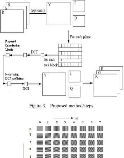
The proposed technique of lossy compression is implemented on color images having 256x256 and 512x512 resolution. The Proposed method is based on the JPEG baseline standard, with no extensions or modifications, so the resulting files are regular JPEGs. The RGB image is read and stored in Matlab software as a 3-dimensional matrix consisting of three 2-3-dimensional matrices, each comprising the respective pixel values of the R, G and B components and then color space conversion is done. Here the image is converted to the YIQ color space from the RGB color space. The 3-D matrix now consists of three Y (luminance), I & Q (Chrominance) matrices. The Y matrix is then taken and divided into 8x8 blocks i.e. blocks containing 8 rows and 8 columns of the Y matrix. The pattern followed here is that first the top leftmost 8x8 block is taken, then move from left to right and then up to down. On each of the blocks 2-dimensional Discrete Cosine Transform is applied. The same process is then carried out on both the chrominance components. Thus we obtain a DCT matrix consisting of the transformed values of all the elements of the original matrix.

The next step in compressing the image is quantizing each element of the transformed matrix. This is done by dividing the 8x8 blocks of the transformed matrix by a quantization matrix of the same size. It separates quantization matrices for the luminance and the two chrominance components. The use of two different matrices is based on the fact that the Human Visual System is more sensitive to luminance as compared to the color components. The chrominance components convey information about color and hence can be quantized more effectively (suppressed more) than the luminance components. In the DCT matrix the low frequency components are present in the top left part of the matrix and the higher frequency components in the lower right part. Eye is most sensitive to low frequencies (upper left corner) and less sensitive to high frequencies (lower right corner), these higher frequency values can be quantized to zero. In the DCT matrix the first element of each 8x8 block will consist of the dc component. This dc coefficient is usually very high in magnitude as compared to the rest of the 63 values. The values obtained from F’ is rounded to nearest integer value.

F`(u,v) = ( , )

( , )

F(u,v): Original DCT coefficient.

Figure 3. Proposed method/steps

Figure 4. The 88 DCT

Quantization of each of the frequency components using a quantization matrix: This is the main stage that causes loss of information. To find the most efficient quantization matrix we first tried to find out on average what the value of the dc coefficient. After implementing the DCT on various images we came to the conclusion that the dc coefficient can range from anywhere between few hundred to about a thousand in magnitude. Since the dc coefficient contains most of the information, it has to be quantized by a very small value. The following quantization matrix was used to quantize the image

Figure 5. Proposed Luminance and Chrominance Quantization Matrix

The DC coefficient is divided by two and the rest of the values are quantized by increasing multiples of two. Next all the values except the top left 4x4 block are increased by a factor of two and applied to the chrominance matrices now to obtain the inverse DCT transform we applied the following

Inverse of DCT is given by: f (x,y) = ∑ ∑ C(u)C(v)F(u, v)cos ( ) cos ( )

for x,y = 0,…..,7, f(x,y) : Element in spatial domain. F(u,v): Original DCT coefficient.

Inverse color transformation applied for converting YIQ to RGB by given expression as R = 1.0*Y + 0.956*I+ 0.621*Q

(IJIRSE) International Journal of Innovative Research in Science & Engineering ISSN (Online) 2347-3207

VI. RESULT AND DISCUSSION

Proposed Method for image compression and decompression is implemented in MATLAB 7. There are various quantitative factors that are calculated as Peak Signal to Noise Ratio (PSNR), Compression Ratio (CR) and Mean Square Error (MSE). Meaning of the above performance measures is as follows:

= 10

I = Image pixel intensity level.

=

= 2 = 1 ( , − , ) 2

Ai = Original image of size M×N Bi = Reconstructed image of size M×N N=Denotes the of pixels in the image σ= Root mean square error

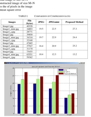
TABLE I. COMPARISON OFCOMPRESSION RATIO

Images File

(bytes) JPEG JPEGmini Proposed Method

Image1.jpg 40328

19.5 22.5 27.3

Image1_mini.jpg 34893 Image1_j.jpg 28771 Image2.jpg 39858

19.7 22.9 24.4

Image2_mini.jpg 34316 Image2_j.jpg 32160 Image3.jpg 47665

16.4 20.9 25.2

Image3_mini.jpg 37547 Image3_j.jpg 31170 Image4.jpg 75455

10.4 12.3 13.2

Image4_mini.jpg 63551 Image4_j.jpg 59362

Figure 6. Comparison of Compression Ratio

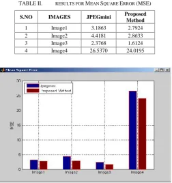
TABLE II. RESULTS FORMEANSQUAREERROR(MSE)

S.NO IMAGES JPEGmini Proposed Method

1 Image1 3.1863 2.7924

2 Image2 4.4181 2.8633

3 Image3 2.3768 1.6124

4 Image4 26.5370 24.0195

Figure 7. Comparison of MSE

REFERENCES

[1] Singh et al., "Multimedia Data Compression Techniques" International Journal of Advanced Research in Computer Science and Software Engineering , October–2013, pp. 321-325,

[2] Asha Lata, Permender Singh;" Review of Image Compression Techniques",ISSN 2250-2459, ISO 9001:2008 Certified Journal, Volume 3, Issue 7, July 2013.

[3] Dr.KishorAtkotiya,ChetanDudhagara;"Jpeg.ImageCompressionAlgorithm",International Journal of Research in Computer Application & Management, Vol No.3, Issue No.03 ISSN 2231-1009 March2013

[4] Manjinder Kaur et al,''A Survey of Lossless and Lossy Image Compression Techniques", International Journal of Advanced Research in Computer Science and Software Engineering, Feb 2013, pp 223-326

[5] Kiran Bindu et.al.,"A comparative study of imagecompression algorithms",International Journal of Research in Computer Science,ISSN 2249-8265 Volume 2 Issue 5 pp. 37-42(2012)

[6] R.Navaneethakrishnan.,"Study of Image Compression Techniques",International Journal of Scientific & Engineering Research, ISSN 2229-5518, Volume 3, Issue 7, July-2012

[7] Sindhu M, Rajkamal R;"Images and Its Compression Techniques",International Journal of Recent Trends in Engineering, Vol 2, No. 4,pp71-75, November 2009

[8] G. K. Wallace, "The jpeg still picture compression standard",Communications of the ACM, Apr. 1991. [9] Chia-Jung Chang, “ Advanced Digital Signal Processing Tutorial”, National University Tiwan.