K- TURBULENCE MODELLING IN COMPUTATIONAL WIND
ENGINEERING FORBUILDINGS
Mohan Kumar.N.S1, SatheeshKumar.K.R.P2
1. INTRODUCTION
Wind produces three unique types of consequences on building: static, dynamic and aerodynamic. The response of load depends on kind of structure. when the structure deflects in reaction to wind load then the dynamic and aerodynamic consequences need to be analysed further to static effect. Sound expertise of fluid and structural mechanics allows in understanding of details of interaction between wind flow and civil engineering structures or buildings. flexible narrow structures and structural elements are subjected to wind triggered along and across the direction of wind. when thinking about the response of a tall building to wind gusts, both alongwind and across wind responses need to be taken into consideration, these arise from different the former being primarily due to buffeting effects caused by turbulence; the latter being primarily due to alternate-side vortex shedding, So it is very important to model turbulence to study the flow over buildings.
1.1 Evolution ofComputational Wind Engineering
Complex fluid flows can be investigated using various tools providedby CFD(computational fluid dynamics). Volume mesh is formed by discretization of spatial domain into small cells.Navier-Stokes equation is reformulated as algebraic equations using numerical methods such as Finite Difference method, Finite Element Method, Finite Volume Method. To simulate the effects of environment these equations are solved numerically over the domain with specified boundary conditions.computers were used in the solution of partial differential equations and by the 1970’s researchers started investigation on using computers for solving fluid flow equations.In 1980’s CFD application stepped into solving wind engineering problems [1] – [2] Great market was there for CFD when it was implemented in few engineering fields and several companies like Fluent, AEA Technology and Computational Dynamics emerged to capture it. Even though there was a great progress in the Computational Wind Engineering, standards for wind loading still relied on wind tunnel studies for design of unconventional buildings [3]. CFD had the great potential to overcome the limitations of wind tunnels. For example, due to Reynolds number limitations modelling of flow inside buildings or bluff bodies in wind-tunnels is difficult. CFD potentially can be integrated with virtual building design process and extract data everywhere in the domain. Critics from the wind engineering community targeted CFD, which is a very young tool that cannot compare with wind tunnels testing that had reached higher level of expertise. On some cases, CFD users have provided different or simply wrong solution at times was reason for the criticism [4]. Like wind tunnel testing CFD also requires expertise and precise guidance. Many attempts were made during 1990’s to provide better and unified guidance for the application of CFD to Wind engineering. CFD codes were developed in the early 2000’s, which were very good at predicting the flow for certain application but failed to offer general codes. In aeronautics industry flow takes place around the streamline bodies, in CWE flow takes place around bluff bodies hence turbulence modelling is particularly important. There was much progress in the last 10 years in CFD for wind engineering problems, it was noted that CFD could be useful to predict global aerodynamic loads on structural elements or could
1 Student. Department of civil Engineering, Kumaraguru College of Technology, Coimbatore, Tamil Nadu, India
2 Assistant professor, Department of Civil Engineering, Kumaraguru college of technology, Coimbatore, Tamil Nadu, India
Abstract- The evolution of computational fluid dynamics over the years in solving wind engineering problems and its ability to predict wind flow over bluff bodies has reached great heights. Researchers are giving great contribution in their respective field in computational wind engineering to achieve great accuracy in wind flow prediction. Development of general codes for prediction of flow over building models are increasing in the past ten years. Turbulence modeling plays a major role in predicting the exactness of the flow along with geometry, domain size and discretization. RANS (Reynolds Averaged Navier - Stokes) model , DNS ( Direct Numerical Simulation ) model , LES ( Large Eddy Simulation ) model, are the models used to solve Basic turbulence equations. This article focuses on the k- turbulence modeling and its application in computational wind engineering. k- model is preffered more than the other models due to its ability predict flows with lesser resources and time efficiency.
Keywords – Building aerodynamics, computational fluid dynamics, CFD, Turbulence modelling, Wind Engineering, flow prediction, Buildings.
complement experimental data on flow generation. CFD had travelled a longway from being redundant in the wind engineering field to providing a complete alternative to conventional wind tunnel testing. CFD in conjunction with wind tunnel helps us to achieve better understanding of flow around buildings and wind loads on structure. CFD needs very careful attention to the following aspects: meshing, turbulence modelling and boundary conditions [5].
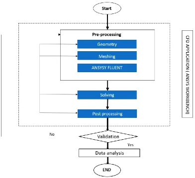
1.2 Methodology
Five steps can be distinguished in the CFD process:
1.2.1 Geometry: The domain and the structure within that domain are built at this step.
1.2.2Meshing: At this key stage, the spatial domain is divided into Control Volumes (CV) to form a mesh (grid)
1.2.3Model set-up: Boundary conditions, turbulence model, material properties, solver settings, data output options, frequency of the output of the flow field, etc are chosen at this stage.
1.2.4Solver: the CFD code discretizes the Navier-Stokes equations, and solves them over the discretized domain of interest. 1.2.5Analysis of results or post-processing where data such as velocity flow fields, vorticity and pressures are extracted on lines, planes, surfaces of the domain under investigation.
1.3 Flow chart for CFD simulation process
Figure 1 Flow chart for CFD simulation process 2 TURBULENCE MODELLING
2.1Introduction
simplicity and computational economy make them the primary choice for commercial applications [6]. It should be stated that DNS, in which the Navier-Stokes equations are solved with none turbulence modelling, cannot be taken into consideration in CWE. this is due to the fact the large 3-d domains and high Reynolds numbers involved might require a quantity of grid points this is beyond current computer capacity. consequently, it is improbable that DNS be used for wind engineering purposes, except a quantum leap in computing power is accomplished.
2.2 Brief History of Turbulence Modelling
The start of the concept of time-averaged Navier-Stokes equations was made by Reynolds in 1895, which had gained a lot of importance with time, and the technique now is often referred as Reynolds averaging. Earliest attempts to model turbulence started with the concept of modelling the turbulent stresses as like the molecular gradient-diffusion process. Boussinesq introduced the concept of eddy viscosity. This concept is well accepted in the fluid dynamics community, although it has no physical basis, and the concept is also called as the Boussinesq approximation. The physics of the viscous flows was still an unknown field until Prandtl postulated the "boundary layer" in 1904. He published his research on turbulence where he came up with computation of eddy viscosity in terms of the mixing length, which was analogous to the mean free path of gaseous molecules. The mixing length hypothesis (now referred as zero-equation model or algebraic model) was the first attempt to model the behaviour of turbulence. Prandtl proposed a model, in which the eddy viscosity depends upon the kinetic energy of the turbulent fluctuations, k. This improvement conceptually accounts for the flow history as it affects the turbulent stresses. This is the begriming of the one equation turbulence models. This concept makes the turbulence model realistic; however, it is unable to provide the turbulent length scale, and is thus "incomplete." In other words, the models still depend upon the flow information to obtain a solution. Ideally, no prior knowledge of any property of the turbulent flow should be required, other than the boundary conditions and the initial conditions, in order to obtain a solution. The first "complete" model, in this sense, was proposed by Kolmogorov [7]. He introduced a second parameter, the rate of dissipation of energy in unit volume and time, co and an additional equation to estimate it. Thus, the two equation models originated. Many researchers started working on the two equation models in the quest for a universal model that could be applied to all types of flows. The most extensive work has been done by Launder and Spalding [2] as the originators of the k-s model, and their successors. The k-s model is the most widely used turbulence model, though many inadequacies have been reported. Chou and Rotta in late 1940s started a completely different stream of models, without using the Boussinesq approximation. Rotta proposed a model with a differential equation for the Reynolds-stress tensor. These types of models are categorized as stress-transport models. For a three-dimensional flow, the stress-transport model introduces seven equations, one for the turbulent scale (length scale or equivalent) and six for the components of the Reynolds-stress tensor. A lot of research work is still going on around turbulence modelling, and new models are being developed and tested. Recent advances in the computational power have led to new techniques such asLES and DNS. The accuracy of turbulence models is improving day by day, with modifications to existing models, and birth of new models and concepts. This section was based on the walkthrough given in Wilcox [8].
2.3 basic concepts
The numerical solution of any fluid mechanics problem requires the solution of the general equations of viscous fluid motion i.e. the continuity equation and the Navier-Stokes equation. These equations are a set of nonlinear partial differential equations with appropriate boundary conditions. The continuity equation and the general form of the Navier-Stokes equations, in tensor notation, are given by:
The first term on left-handside is the instantaneous acceleration termfollowed by the convection term. The first term on the right-hand side is the pressure gradient term followed by the viscous dissipation term. F denotes the body forces. For incompressible flows is constant and the equations are simplified.
2.4 Turbulent Flow Models in ANSYS FLUENT
ANSYS FLUENT provides the following choices of turbulence models: Spalart-Allmaras model
k- models
Standard k- models
Renormalization-group (RNG) Standard k- models Realizable Standard k- model
k- models
Standard k- model
Shear-stress transport (SST) k- model
Transition k-kl- model Transition SST model
Reynolds stress models (RSM)
Linear pressure-strain RSM model Quadratic pressure-strain RSM model Low-Re stress-omega RSM model
Detached eddy simulation (DES) model, which includes one of the following RANS models. Spalart-Allmaras RANS model
Realizable Standard k- models RANS model
SST k- RANS model
Large eddy simulation (LES) model, which includes one of the following sub-scale models. Smagorinsky-Lilly subgrid-scale model
WALE subgrid-scale model Dynamic Smagorinsky model
Kinetic-energy transport subgrid-scale model
3 TYPES OF K- TURBULENCE MODELS
3.1 Standard k- models
The standard k- model of Launder and Spalding [2] is by far the most popular and most widely used turbulence model. It is a semi-empirical model and consists of two transport equations. One for the specific turbulent kinetic energy (k) and one for the turbulent dissipation rate ( ).
Transport Equations
3.2 The RNG k- Model
A variant of the standard k- model is derived from the instantaneous Navier-Stokes equation using a mathematical technique called "renormalization group" (RNG) methods. The model resulting based on analytical derivation is different from the standard k- model in constants and some additional terms and functions in the transport equations for k and [10]. Detailed information about the renormalization group method and the RNG k- model given by Yakhot and Orszag [9].
Transport Equations
3.3 The Realizable k- Model
The realizable k- model is yet another variation of the standard k- model proposed by Shih, Liou, Shabbir and Zhu [11]. The term "realizable" reflects model's ability to satisfy mathematical constraints on normal stresses and remain consistent with the physics of turbulence. This is achieved by making the term Cµ variable instead of keeping it constant. Also, the dissipation rate calculations are enhanced by using new eddy-viscosity formula with variable Cµand a new transport equation for based on the dynamic equation of the mean-square vorticity fluctuation [10].
(3.1
)
(3.2)
(3.3
)
(3.4)
Transport Equations
4 APPLICATION OF THE K- MODEL TO CWE
The standard k- turbulence model has been widely used in various applications for its efficiency. However, the standard version is not exempt from drawbacks in CWE. Early work has shown a major limitation: the standard k- turbulence model clearly over-predicts the turbulence kinetic energy, k, in the impinging region, i.e. around the frontal corners of the bluff bodies [13] – [15]. This leads to poor prediction of the flow on the roof, so that separation does not occur as it should [4]. In addition, the stagnation point on the windward face is not accurately predicted. The over-prediction ofturbulent kinetic energy is believed to be due to the use of Eddy Viscosity Modelling [15].To reduce the over production of k in the impinging region, several research groups have proposed revised versions of the standard k- model. The most renowned of these models are the Launder-Kato(LK)model [16] and theMurakami-Mochida-Kondo (MMK) model [12]. The LK k- model helps to significantly reduce the production of k, but inconsistency in its mathematical formulation lead to the development of the MMK k- model.Another modified version of the standard k- model must be mentioned here, The RNG k- model[17]. In short, the model removes the effects of the smaller scales from the transport equations and expresses their effects in terms of larger scale motions and a modified viscosity to account for a wider range of motion scales [18]. At first, this model was very promising because of the advanced mathematical techniques involved and was therefore investigated in CWE. However, this interest has rapidly decreased as research groups have noticed mixed results [19]-[21]. In 2002, Richards and Quinn reviewed the performance of the standard k-c, the MMK k-e and the RNG k-c model for modelling the flow around a cube. They compared the numerical results obtained by other research groups to full-scale data recorded at the Silsoe cube, which is a 6-meter square cube installed at the Silsoe Research Institute in Bedford. The authors noticed that the MMK model predicts an excessive separation, whereas the standard k-e model predicts no separation at all and the RNG k-e model can predict a correct separation and an acceptable reattachment length. However, when the wind was applied at a 45° angle to the cube, none of these models were able to predict the correct pressure distribution on the cube, especially the negative pressure along the windward edges. It was concluded that none of the models were able to predict the correct turbulence levels, and that velocities are better predicted than the pressure distribution. More specifically all the models under-predict the pressures on the roof [4].
5.COMPARISION OF K- TURBULENCE MODELS
Type of k- models Advantages Disadvantages
Standard k- models Robust,
economical,
reasonably accurate,
long accumulated performance data.
Mediocre results for complex flows with severe pressure gradients,strong streamline curvature, swirl and rotation. Predicts that round jets spread 15% faster than planar jets whereas they spread15% slower.
RNG k- Model
Good for moderately complex
Behaviour like jet impingement
separating flows,
swirling flows, and
secondary flows
Subjected to limitations due To isotropic eddy viscosity assumption. Same problem with round jets as standard
k-Realizable k- Model Offers largely the same benefits as RNG but also resolves the round jet anomaly.
Subjected to limitations due To isotropic eddy viscosity assumption.
6. CONCLUSION
encountered in these situations. The turbulence models did not predict the separation bubble and reattachment on the roof, which causes overprediction of turbulence kinetic energies in the areas with high velocity gradients like the flow near the leading edge of the roof and side surfaces. This overprediction is not adequately balanced with dissipation of turbulence resulting in inaccurate prediction of the turbulent viscosity, which is comparatively low on the windward face and high in the separation and recirculation regions. This, in turn, causes nigh suction pressures on roof and sides and only shows good agreement with the experimental data on the windward face. Overall performance of the realizable k-s model was consistent and better than the other four models. The RNG k-s model predicted the highest drag and lowest lift on the building model, while the standard k-s model predicted the lowest drag and highest lift on the building.
7. REFERENCES
[1]. S. V. Patankar and D. B. Spalding. A calculation procedure for heat, mass and momentum transfer in three-dimensional parabolic flows. Int. J. Heat Mass Transfer, 15: 1787, 1972.
[2]. B. E. Launder and D. B. Spalding. The numerical computation of turbulent flows. Com- put. Methods Appl. Mech. Eng., 3: 269-289,1974.
[3]. Theodore Stathopoulos. Computational wind engineering: Past achievements and future challenges. Journal of Wind Engineering and Industrial Aerodynamics, 67-68: 509-532, 1997.
[4]. P. J. Richards and A. D Quinn. A6m cube in an atmospheric boundary layer flow part 2. computational solutions. Wind and Structures, 5(2-4): 177-192,2002.
[5]. Ian P. Castro and J. M. R. Graham. Numerical wind engineering: the way ahead? In Proceedings of The Institution of Civil Engineering Structures &Buildings, pages 275-277, August 1999.
[6]. Kemal Hanjalic and Sasa Kenjeres. Some developments in turbulence modelling for wind and environmental engineering. Journal of Wind Engineering and Industrial Aerodynamics, 96: 1537-1570,2008.
[7]. A. N. Kolmogorov. The local structure of turbulence in incompressible viscous fluid for very large Reynolds numbers. In Dokl. Akad. Nauk SSSR, volume 30, pages 9-13, 1941.
[8]. Wilcox D.C., Turbulence Modelling for CFD, Second Edition, DCW Industries, Inc., (2002).
[9]. Yakhot V., Orszag S.A., "Renormalization group analysis of turbulence, I Basic Theory", Journal of Scientific Computing, Vol. 1, No. 1, (1986). [10].Fluent 12.0 Users Guide, Fluent Inc (2009)
[11].Shih T.-H., Liou W.W., Shabbir A., Zhu J., "A new k-s eddy-viscosity model for high Reynolds number turbulent flows - Model development and validation", Computers Fluids, Vol. 24, No. 3, (1995), Pp. 227-238.
[12].S. Murakami, A. Mochida, K. Kondo, Y. Ishida, and Tsuchiya. Development of new k-epsilon model for flow and pressure fields around bluff body. Journal of Wind Engineering and Industrial Aerodynamics, 67&68: 169-182,1994.
[13].S. Murakami and A. Mochida. On turbulent vortex shedding flow past 2d square cylinder predicted by cfd. Journal of Wind Engineering and Industrial Aerodynamics, 54-55: 191-211,1995.
[14].S. Murakami. Current status and future trends in computational wind engineering. Journal of Wind Engineering and Industrial Aerodynamics, 67&68: 3-34,1997.
[15].S. Murakami. Overview of turbulence models applied in cwe-1997. Journal of Wind Engineering and Industrial Aerodynamics, 74-76: 1-24,1998. [16].M. Kato and B. E. Launder. The modelling of turbulent flow around stationary and vibrating square cylinders. Prep. of 9th Symp. On Turbulent shear
flow, 157: 10-4-1- 6,1993.
[17].V Yakhot, S. A. Orszag, S. Thangam, T. B. Gatski, and C. G. Speziale. Development of turbulence models for shear flows by a double expansion technique. Physics of Fluids A, 4: 1510-1520,1992.
[18].H. K. Versteeg and W. Malalasekera. An Introduction to Computational fluid dynamics, The Finite Volume Method. Pearson Education, 2007. [19].S. Swaddiwudhipong and M. S. Khan. Dynamic response of wind-excited building using cfd. Journal of Sound and Vibration, 253(4): 735-754,2002. [20].R. P. Hoxey, P. J. Richards, and J. L. Short. A6m cube in an atmospheric boundary layer flow part 1. full-scale and wind-tunnel results. Wind and
Structures, 5(2-4): 165-176, 2002.
[21].A. Mochida, Y. Tominaga, S. Murakami, R. Yoshie, T. Ishihara, and R. Ooka. Comparison of various k-epsilon models and dsm applied to flow around a high-rise building - report on air cooperative project for cfd prediction of wind environment -. Wind and Structures, 5(2-4): 227-244,2002. [22].Durbin P.A., Medic G., Seo J.-M., Eaton J.K., Song S., "Rough wall modification of two-layer k-s". Transactions of the ASME, Vol. 123, (2001), pp.
16-21