http://www.sciencepublishinggroup.com/j/sjams doi: 10.11648/j.sjams.20170504.14
ISSN: 2376-9491 (Print); ISSN: 2376-9513 (Online)
On Maximum Likelihood Estimation for the Three
Parameter Gamma Distribution Based on Left Censored
Samples
Etienne Ouindllassida Jean Ouédraogo
1, *, Blaise Somé
1, Simplice Dossou-Gbété
21Laboratory of Numerical Analysis, Informatics and Bio-mathematics (LANIBIO), Unit of Formation and Research in Exact and Applied
Sciences, University of Ouagadougou, Ouagadougou, Burkina Faso
2Laboratory of Mathematics and Their Applications of Pau (LMAP), University of Pau and Pays de l’Adour, Pau, France
Email address:
[email protected] (E. O. J. Ouédraogo)
*Corresponding author
To cite this article:
Etienne Ouindllassida Jean Ouédraogo, Blaise Somé, Simplice Dossou-Gbété. On Maximum Likelihood Estimation for the Three Parameter Gamma Distribution Based on Left Censored Samples. Science Journal of Applied Mathematics and Statistics.
Vol. 5, No. 4, 2017, pp. 147-163. doi: 10.11648/j.sjams.20170504.14
Received: May 30, 2017; Accepted: June 14, 2017; Published: July 24, 2017
Abstract:
This paper deals with a Maximum likelihood method to fit a three-parameter gamma distribution to data from an independent and identically distributed scheme of sampling. The likelihood hinges on the joint distribution of the n − 1 largest order statistics and its maximization is done by resorting to a MM-algorithm. Monte Carlo simulations is performed in order to examine the behavior of the bias and the root mean square error of the proposed estimator. The performances of the proposed method is compared to those of two alternatives methods recently available in the literature: the location and scale parameters free maximum likelihood estimators (LSPF-MLE) of Nagatsuka & al. (2014), and Bayesian Likelihood (BL) method of Hall and Wang (2005). As in several papers on the three-parameter gamma fitting (Cohen and Whitten (1986), Tzavelas (2009), Nagatsuka & al. (2014), etc.), the classical dataset on the maximum flood levels data in millions of cubic feet per second for the Susquehanna River at Harrisburg, Pennsylvania, over 20 four-year periods from 1890–1969 from Antle and Dumonceaux’s paper (1973) is consider to illustrate the proposed method.Keywords: Estimation, Likelihood, MM-algorithm, Order Statistics, Pearson Type III Model,
Three-Parameter Gamma Model, Left Censoring1. Introduction
In many fields of science and technology one must carry out the statistical analysis of skewed numerical datasets. In the field of reliability (lifetime study) or hydrology (annual maximum flows or streamflows study) (refer to Bobee and Ashkar (1991), [1] for example), it is common to deal with skewed data made of recorded values that cannot fail below a threshold. One of the statistical model appropriate for statistical analysis of such dataset is the three-parameter gamma model of probability distributions. A probability distribution that obeys to the three-parameter gamma model is identified by a vector ∈ ℝ , = , , and is defined by a probability density function (pdf) f (with respect to the Lebesgue’s measure) as follows:
, = − − − 1 ,
The parameter ν ∈ ℝ denotes the threshold value and is called the location parameter; β > 0 is the scale parameter and λ> 0 is the shape parameter. Let ⊂ ℝ be the parameter space. If 0< λ≤1, the distribution is reverse ‘‘J’’ shaped, whereas if λ > 1, the distribution is bell-shaped and its mode is equal to ν+ (λ − 1)β [2]
situations can then arise when the maximum likelihood method is used to fit the model to data. Let’s notice first that the likelihood is unbounded for values of the shape parameter λ smaller than 1 as ν is unknown and goes towards the observed sample value x. Non-existence of a global optimum of the log-likelihood in a certain range of the parameters’ values, convergence problems and large variability of the
parameters’ estimates are main limitations with the use of the maximum likelihood method. The non-regular behavior of the maximum likelihood method for the three-parameter gamma model has been addressed from theoretical statistics point of view in several works and one can refer to the paper by Nagatsuka & al. (2014), [3], for a concise and clear overview of the main results on this topic. Several works including Bowman and Shenton (2002),
Cheng and Iles (1987, 1990), Smith (1985), Cohen and Whitten (1982) [4, 5, 6, 7, 2] have aimed to provide reliable estimates of θ for the three-parameter gamma distribution. In the recent past some studies were carried out to provide the conditions which the data must check to make it possible to overcome some of the difficulties encountered in the use of the maximum likelihood method. As an example, Tzavelas (2008) [8] provides with conditions on the data under which the root of the score equations exists. These conditions hinges on the third central empirical moment µ̂3. If µ̂3<0, the score function has at least one root. By cons, µ̂3>0 yields two possibilities: either the score function has no root or it has at least two roots. In spite of a lack of sharpness, these results are of a practical range insofar as they are related to the dataset. Others works including Balakishnan (2000), Hall and Wang (2005),Tzavelas (2009), Nagatsuka and al. (2014), [9, 10, 11, 3], have developed methods that aim to provide with reliable estimators as those based on complete and censored samples and order statistics.
In this article, a new estimation method using the likelihood based on the n − 1 largest values of a sample of size n from a three-parameter Gamma distribution is develop. An MM algorithm [12] is providing to determine Maximum Likelihood Estimates (MLEs) of θ. The performance of the methodology developed is assessed by a simulation study and illustrated with a numerical real-life example.
The rest of the paper is organized as follows. The next section presents the likelihood function of the parameters vector θ and the third section deals with a MM approach for its maximization. The results of a Monte-Carlo study carried out for the evaluation of the performance of the estimator of θ is presented in the fourth section. The last section is devoted to a discussion.
2. Model Fitting Method
2.1. An Order Statistics Based Likelihood
Given an independent and identically distributed (i.i.d) sequence : , let F(x∣θ) be the cumulative distribution function (cdf) and denotes (Xi:n)i=1:n the associated sequence of order statistics.
! , = " #| %#
The joint density of the sequence (Xi:n)i=2:n is therefore defined by
&':( ')*:( #,
= +! ! #-| .
-# | 1 /0*1021...10( #
where # , #-, . . . , # is a strictly increasing sequence. Let : denote a sample of size n from a three-parameter gamma distribution with unknown three-parameters vector θ and (xi:n)i=1:n is the non-decreasing sorted values. The likelihood function based on last n − 1 order statistics is defined as follow:
4 | : , 5 = 2: + = +! ! -: | .
-: |
Taking the logarithm of both sides leads to the following log-likelihood function for left censored data
7 | -: , ⋯ , :
7 | -: , ⋯ , : = 79: +! − + 79: − +79:; < + > 79:
?
-?: −
− > 79: ?
-?: − −1> ?: − ?
-+ 79: -: −
+ 79: " #
@ −
1
-: − #%#
2.2. MM-algorithm Approach to the Maximization of an Objective Function
The acronym MM stands for Majorization-Minorization or Minorization-Maximization algorithm (Lange (2000, 2004, 2013), [12, 13, 14]). Now, let us focus on Minorization-Maximization version of the MM approach to computing the argument value where an objective function reaches a local maximum. Let’s consider the problem of maximization of a function Ψ whose domain is X. This procedure relies on the concept of surrogate function, which is maximized instead of the objective function at each iteration of the algorithm. The starting point of a MM-algorithm consists looking for a function Q, named a minorization function, defined on the cartesian product X × X and such that: ∀(x, x0) ∈ X × X, Ψ(x) ≥ Q(x∣x0) and B @ = C @| @ . It comes from the above property that forall @, ∈ × ,
C | @ ≥ C @| @ ⇒ B ≥ C | @ ≥ B @
function Q that is easy to deal with. The surrogate function for minorization is chosen by resorting to inequalities of mathematical analysis as Arithmetic or Geometric Mean inequality, Cauchy-Schwarz inequality, Jensen’s inequality, minimization via supporting hyperplane, etc. Although the surrogate functions can be defined in many different ways, what should be bear in mind is that they define pointwise lower-bound of the gap between two values of the objective function Ψ.
Once the minorization function Q is available, a MM-algorithm consists in cycling between two steps until some stopping criterion is fulfilled as follows:
(1).Compute → C | H for H fixed; this step stands for the E-step of an EM-algorithm.
(2).Update xt − 1 as xt=argmax{Q(x∣xt − 1),x ∈ X}; this maximization step is the analog of the Maximization step of an EM-algorithm.
Therefore, starting at an initial value @, the update scheme shown above produces a sequence H H ∈ ℕ in X such that
B H ≤ B H B H+ 1 = C H | H
It comes a sequence H H∈ ℕ could be carried out, a cluster point of which might be a local maximum for the function Ψ (i.e. a stationary point for Ψ). The convergence of the MM-algorithm has been addressed in several books and survey papers including Wu (1983), Lange (2013) and Vaïda (2005) [15, 14, 16]. General conditions of convergence were provided in the book by Lange (2013) [14] and Vaida (2005) has established some additional one [16].
3. Derivation of a MM-algorithm for
Minorizing the Left Censored Data
Log-Likelihood
The design of a MM-algorithm is based on a wise choice of minorizing function to obtain a simple lower bound for the log-likelihood function. In the subsection below, the minorizing function for our log-likelihood is derived.
3.1. Derivation of a Function Minorizing the Log-Likelihood
Let’s denote:
7 | -: , ⋯ , : = −+ 79: − +79:; <
+ > 79: ?
-?: − + 79: -: − − > 79: ?
-?: −
−1> ?: − : ?
-− K+ − 1L : −
7- | -: , ⋯ , :
= 79: M" #
@ M−
-: − #N %#N
One has
7 | -: , ⋯ , : = 79: +! + 7 | -: , ⋯ , : + 7- | -: , ⋯ , :
7 | -: , ⋯ , : ≥ C | ′, : , ⋯ , :
= C | ′, : :
where
C | ′, : : = −+79:; < + + ;1 − 79: ′ <
+ > 79: ?
-?: − ′ + > : − ′ ?: − ′ ?
-+ M79: -: − ′ + : − ′ -: − ′N
−2 ′ P+ + >- : − ′ ?: − ′ ?
-+ : − ′ -: − ′Q
− 2′ : − ′ -: − - P>
: − ′ ?: − ′ ?
-+ : − ′ -: − ′Q
− + − 12 ′ : − -: − ′ + >
1 ?: − ′ ?
-− + ′2 ′-
-−1> ?: − : ?
-− + − 1 ′2 - : − ′
− > 79: ?
-?: − ′ − ′ > 1 ?: − ′ ?
-See Appendix 7.2 Let’s denote:
R@ = " #
@ −
-: − #%#
R =R 1
@ " 79:@ # # M−
-: − #N %#
R- =R 1
@ " #@ M−
-: − #N %#
One has
7- | -: , ⋯ , : ≥ C- | ′, -: , ⋯ , :
where
C- | ′, -: , ⋯ , : = R ′ −R- ′ -: − -2 ′ -: − ′
See Appendix 7.3 Since
7 | -: , ⋯ , : = 79: +! + 7 | -: , ⋯ , : + 7- | -: , ⋯ , :
one has
7 | -: , ⋯ , : ≥ 79: +! + C | ′, : : + C- | ′, -: , ⋯ , :
and the following statement holds
7 | -: , ⋯ , : ≥ 79: +! + C | ′, : :
where
C | ′, : :
= C | ′, : :
+ C- | ′, -: , ⋯ , :
Moreover if SC | ′, : : denotes the
gradient vector of the function → C | ′, : : one has
SC | ′, : : = S7 ′| -: , ⋯ , :
From previous results, one may note that the obtained Q-function takes into consideration the “n” complete data although the original log-likelihood function is based on the “n-1” largest data.
3.2. Computational Procedure: Maximization Algorithm
3.2.1. Preliminaries
TC | ′, : :
T
= −+ UV
+ ′W1 +1+ P>? - ?: : − ′− ′+
: − ′ -: − ′QXY
−+ 79: ′ − 1 + > 79: ?
-?: − ′ + 79: -: − ′
+ > : − ′ ?: − ′ ?
-+ : − ′ -: − ′ + R ′
where λ→ψ(λ) is the digamma function
TC | ′, : :
T = − ′ : − ′
-: − P
: − ′ -: − ′
+ > : − ′ ?: − ′ ?
-Q
+1
′ + − 1: − ′: − +
R- ′ -: −
-: − ′ + > 1 ?: − ′ ?
-TC | ′, : :
T = −+ ′′2 + 1->? - ?: − : +1 Z + − 1 ′ : − ′ + ′ -: − ′ R- ′ [
TC | ′, : :
T =−1\+ ′′- ]− > ?: − : ?
^
−1 Z− ′ + − 1 : − ′ + -: − ′ R- ′ [
The function → C | ′, : : is concave and thus admits a unique global maximum for any θ′ fixed.
Hessian matrix of the function → C | ′, : : is diagonal with nonzero components
T-C | ′,
: : T -= −+ UTVT
+1′ \1 +1+ P> : − ′ ?: − ′ ?
-+ : − ′ -: − ′Q^Y
T-C | ′, : :
T - = −1′ M + − 1: − ′ + R-: - − ′N′
−3 ′ : − ′ -: − ] \
: − ′ -: − ′ + >
: − ′ ?: − ′ ?
-^
T-C | ′,
: :
T - = −+ ′′-− 2 > ?: − : ?
-− 3]Z + − 1 ′ : − ′ + ′ -: − ′ R- ′ [
3.2.2. Updating Scheme
Algorithm 1: Parameters’ updating scheme Require: `, a = b a, a, a
Output: ` + 1, a+ 1 = b a+ 1, a+ 1, a+ 1 Do: until a stopping criteria is fulfilled:
(1). a+ 1 = b , a, a
(2). a = cd:ec f@C a | a
ag= b a , a, a ,
(3). a = b a+ 1, , a
(4). a = cd:ec hf@C a+ 1 | ag
agg= b a , a , a ,
(5). a = b a , a ,
(6). a = cd:ec 1 i:(C a | agg k=k + 1
3.2.3. Updating Step for the Location Parameter One can write
TC | ′, : :
T = + − 1: − ` : − | ′
where
` #| ′ = − ′ + − 1: − ′ -\> : − ′ ?: − ′ ?
-+ : − ′ -: − ′^
+1
+ − 1 \>? - ?: 1− ′+
R- ′ -: − ′ -: − ′ ^ #
]
+ j ′ 1
: − ′ +
R- ′
+ − 1 ′ -: − ′ k #
To solve the equation
TC | ′, : :
T = 0
is equivalent to ` : − | ′ = 0. It is readily seen that k is a monotonically increasing function on the domain 0, +∞ since R- ′ > 0 and ?: − ′ > 0
for r≥1. Moreover
75e
0→@,0f@` # = −
′ : − ′
-+ − 1 \>? - ?: : − ′− ′+
: − ′ -: − ′^ < 0
and limu→ + ∞k(u)= + ∞. Thus the equation k(u)=0 has an unique solution in 0, +∞ and the same for the equation
TC | ′, : :
T = 0 ∈ −∞, : .
3.2.4. Updating Step for the Scale Parameter
TC | ′, : :
T = − 1 : | ′
and
: | ′, : : =+ ′
]
′- − > ?: − : ?
− ′Z + − 1 : − ′ + -: − ′ R- ′ [
The assertion
TC | ′, : :
T = 0
holds if and only if g(β∣θ′, (xi:n)i=1:n)=0, the latter being equivalent to finding root of the function β→g(β∣θ′, (xi:n)i=1:n). The derivative g′(β∣θ′, (xi:n)i=1:n) of this function is equal to 0 if
= p4 ′ \′- + >1 ?: − : ?
^
2
Let
@= p ′
-4 ′ \1+ >? ?: − : ^
2
one notices that :′ | ′, : : is positive if > @ and negative in the left side of @. Since R- ′ > 0,
: 0| ′, : : = − ′; + − 1 : − ′ < − ′ -: − ′ R- ′ < 0
and it follows that : @| ′, : : is also negative. Therefore the unique solution of the equation
TC | ′, : :
T = 0
belongs to the interval @, +∞ .
3.2.5. Updating Step for the Shape Parameter
TC | ′, : :
T = −+ UV
+ ′\1 +1+ P>? - ?: : − ′− ′+
: − ′ -: − ′Q^Y
+ > 79: ?
-?: − ′ + 79: -: − ′ + > : − ′ ?: − ′ ?
-+ : − ′
TC | ′
T = 0
is equivalent to find the roots of the function
ℎ | ′, : :
= V + ′ ′| : :
+ b | : :
where
′| : : = 1 +1+ P> : − ′ ?: − ′ ?
-+ : − ′ -: − ′Q
and
b ′| : : = 79: ′ − 1
−1+ \> 79: ?
-?: − ′ + 79: -: − ′ ^
−1+ \> : − ′ ?: + − ′ ?
-+ : − ′
-: − ′ + R ′ ^
h is increasing function of λ on 0, +∞ . Since p(θ′|(xi:n)i=1:n) is positive, the function h has the same limites as the digamma function which tends to − ∞ and + ∞ as λ tends respectively to 0 and + ∞. Hence the function → ℎ | ′, : : has an unique root in the interval 0, +∞ and the same for the solution of the equation
st u|ug, ':( ')i:(
s = 0.
From now on, the estimation method which corresponds to the algorithm exposed in this section will call Maximum Marginalized order statistics Likelihood (MMosLE).
4. Simulation Study for an Empirical
Evaluation of the Proposed Estimators
A simulation study has been carried out to evaluate the performance of the estimators of the MMosLE method, the results of which is reported hereafter. These simulations was run by considering the same configurations of the three-parameter gamma model of probability distribution as Nagatsuka & al. (2014), [3], by selecting the following values of the shape parameter λ: 0.5, 1.0, 2.0, 3.0, and 4.0 when the location and the scale parameters are taken fixed as ν=0 and β=1. The performance of the estimators is evaluated through the bias and root-mean-squared error (RMSE). The performance statistics of the proposed estimators are thus compared to these reported in the paper by Nagatsuka & al. (2014), [3], for Location and Scale Parameters Free Maximum Likelihood method (LSPF-MLE) and the Bayesian Likelihood (BL) method proposed by Hall and Wang (2005) in [10], In addition, as in the paper by Nagatsuka & al. (2014), [3], joint bias of the three parameters as well as their joint mean squared error are compute in order to evaluate the marginal performance on mean squared error (MSE) of the estimators of the three parameters. The joint bias is sum of the absolute values of the bias and the joint MSE is the trace of the MSE matrix of the estimators.
Since iterative algorithms depend on the choice of the initial value, two initializations step were tested. The first is deterministic while the second, based on the empirical moments, is stochastic. For the implementation of the later, many different initial values were trying and choose the solution that has the highest converged likelihood value. Both results will labeled MMosLE(1) and MMosLE(2) respectively. In the absence of precision, the results presented in the following will be those obtained with MMosLE(2) initialization step. All computations were carried out with R computing environment (R Core Team, (2015), [17]) and data were generated by the use of the package PearsonDS (Becker and Klössner, (2013), [18]).
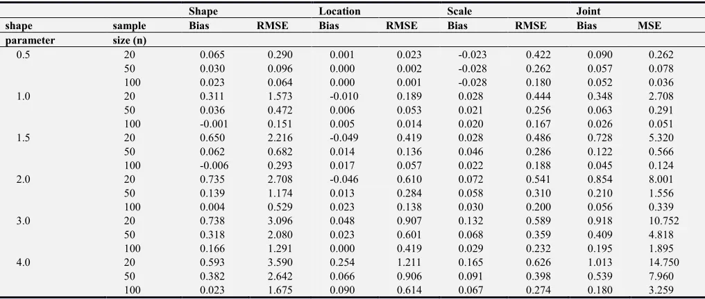
Table 1. Estimated bias, RMSE, and joint MSE based on 1000 simulations.
Shape Location Scale Joint
shape sample Bias RMSE Bias RMSE Bias RMSE Bias MSE
parameter size (n)
0.5 20 0.065 0.290 0.001 0.023 -0.023 0.422 0.090 0.262 50 0.030 0.096 0.000 0.002 -0.028 0.262 0.057 0.078 100 0.023 0.064 0.000 0.001 -0.028 0.180 0.052 0.036 1.0 20 0.311 1.573 -0.010 0.189 0.028 0.444 0.348 2.708 50 0.036 0.472 0.006 0.053 0.021 0.256 0.063 0.291 100 -0.001 0.151 0.005 0.014 0.020 0.167 0.026 0.051 1.5 20 0.650 2.216 -0.049 0.419 0.028 0.486 0.728 5.320 50 0.062 0.682 0.014 0.136 0.046 0.286 0.122 0.566 100 -0.006 0.293 0.017 0.057 0.022 0.188 0.045 0.124 2.0 20 0.735 2.708 -0.046 0.610 0.072 0.541 0.854 8.001 50 0.139 1.174 0.013 0.284 0.058 0.310 0.210 1.556 100 0.004 0.529 0.023 0.138 0.030 0.200 0.056 0.339 3.0 20 0.738 3.096 0.048 0.907 0.132 0.589 0.918 10.752
50 0.318 2.080 0.023 0.601 0.068 0.359 0.409 4.818 100 0.166 1.291 0.000 0.419 0.029 0.232 0.195 1.895 4.0 20 0.593 3.590 0.254 1.211 0.165 0.626 1.013 14.750
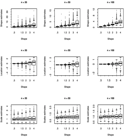
4.1. Variability of Estimates
The boxplots in Figure 1 show that all the parameters’ estimators have a skew distribution when the sample size is small or medium. The skewness increases as the magnitude of the actual value of shape parameter increases. Therefore the asymptotic normality property cannot be considered if the sample sample size is not large enough.
4.2. Monte Carlo Estimation of the Performance Metrics of the MMosLE Method
The aim of this section is to discuss the performances of the MMosLE based on simulated datasets corresponding to the six configurations of the three-parameter gamma model of probability distribution stated at the beginning of the section. The discussion is based on the bias and the root mean squared error estimated using simulated dataset.
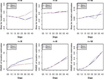
Figure 2. Effect of initialization steps on shape parameter estimates based on 1000 simulated samples.
Both initialization steps provide a positive bias for the shape parameter. Moreover, the magnitude of the bias is comparable when sample size is moderate or large (n≥50). This statement is also valid for the root-squared-errors metric. For small sample size (n≤20) against, graphics suggest that the MMosLE (2) initialization step is more efficient in terms of bias and root-squared-errors.
For small sample size (n≤20), bias of location parameter estimator is positive when MMosLE(2) initialization step is used whilist that of MMosLE(1) initialization step is negative. However, the magnitude of bias is comparable in absolute value. In terms of root-squared-errors, MMosLE(2) initilization step outperfoms its competitor. For moderate or large sample size(n≥50), both initialization steps are comparable.
Figure 4. Effect of initialization steps on scale parameter estimates based on 1000 simulated samples.
No significative differences between metrics obtained with both initialization steps. Bias and RMSE of the scale parameter increase when the actual value of the shape parameter is large.
Although the performances of the estimator evaluated through the estimation of the bias and the root mean squared errors are not strong for the samples of small size (approximately 20 or less) one can note that these performances improve quickly starting from modest sizes of sample (around 50). Indeed the bias and the root mean squared errors of the estimates of the three parameters improve as the sample size increases.
4.3. Performance Metrics Estimated by Monte Carlo Simulations for Two Alternative Methods
Let us start by giving a brief description of two estimation methods discussed in the recent literature on the fitting of three-parameter gamma distribution to skew dataset. One of these estimation procedure is the so-called Location and Scale Parameters Free Maximum Likelihood method (LSPF-MLE) of Nagatsuka, Balakrishnan and Kamakura (2014), [3])., while the other is the Bayesian likelihood method (BL) of Hall and Wang (2005), [10]).
4.3.1. Location and Scale Parameters Free Maximum Likelihood Method
Given an iid sequence : from a three-parameter gamma distribution, let’s considers the statistics
v: = : − :
: − : , 5 = 1, ⋯ , +
The LSPF-MLE method is performed in two steps as follows:
step 1: Since the distributions of W1:n’s depend only on the shape parameter λ and this one is estimated by maximizing the likelihood of λ based on the sequence v: -: . step 2: let’s denote ^ H= : and
^ H= 1
+^> − ^ H
The location and the scale parameters are estimated as follows:
^ = : − ̂^ H" y1 − !; |^, 1,0<z
@ %
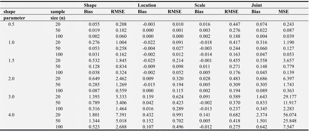
Table 2. Location and Scale Parameters Free MLE(LSPF-MLE) method: estimated bias, RMSE, and joint MSE based on 1000 simulations from Nagatsuka and al. (2014).
Shape Location Scale Joint
shape sample Bias RMSE Bias RMSE Bias RMSE Bias MSE
parameter size (n)
0.5 20 0.055 0.208 -0.003 0.010 0.016 0.447 0.074 0.243 50 0.019 0.102 0.000 0.001 0.003 0.276 0.022 0.087 100 0.002 0.060 0.000 0.000 0.002 0.188 0.004 0.039 1.0 20 0.276 1.004 -0.022 0.091 -0.018 0.417 0.316 1.190 50 0.053 0.258 -0.004 0.027 -0.003 0.244 0.060 0.127 100 0.031 0.162 -0.002 0.012 -0.014 0.163 0.047 0.053 1.5 20 0.532 1.845 -0.025 0.214 -0.001 0.455 0.558 3.657 50 0.128 0.834 -0.009 0.098 0.011 0.271 0.148 0.779 100 0.038 0.324 -0.002 0.052 0.005 0.176 0.045 0.139 2.0 20 0.649 2.462 0.009 0.320 0.028 0.483 0.686 6.397 50 0.285 1.269 -0.015 0.194 0.005 0.309 0.305 1.743 100 0.087 0.559 0.000 0.115 0.002 0.194 0.089 0.363 3.0 20 1.393 5.333 0.159 0.624 0.091 0.589 1.643 29.177
50 0.789 3.406 0.042 0.423 -0.002 0.370 0.833 11.917 100 0.316 1.464 0.016 0.289 -0.013 0.237 0.345 2.283 4.0 20 1.801 7.391 0.432 0.991 0.141 0.682 2.374 56.074
50 1.344 5.018 0.152 0.702 0.005 0.418 1.501 25.848 100 0.523 2.688 0.107 0.496 -0.012 0.275 0.642 7.547
4.3.2. Bayesian Likelihood Method
The bayesian likelihood method studied by Hall and Wang (2005), [10], considers the density functions of the form
ℎ | , { = − : − |{ 1 , where
limy→0g(y∣φ) is a positive constant and λ>0. Therefore the likelihood may be unbounded for 0<λ<1. The density function of the three-parameter gamma distribution belongs to this class of density functions. Let’s denote : : the order statistics of a sample : drawn from a three parameter gamma distribution, Hall and Wang’s method hinges on the maximization of the penalized likelihood
7 + | : , ⋯ , : = : −
-: − . : |
The factor (x1:n − ν)/(x2:n − ν), an empirical prior for ν, shifts the estimator of ν from the value x1:n which is known to be an overestimate to a more plausible value that is smaller than : .
Numerical summary in Table 3 result from Monte Carlo simulations carried out by Nagatsuka and al. (2014) [3] with
the aim of comparing performances of the LSPF-MLE estimators with those of the BL method.
Table 3. Bayesian Likelihood(BL) method: estimated bias, RMSE and joint MSE based on 1000 simulations from Nagatsuka and al. (2014).
Shape Location Scale Joint
shape sample Bias RMSE Bias RMSE Bias RMSE Bias MSE
parameter size (n)
0.5 20 0.067 0.204 0.001 0.008 -0.025 0.412 0.093 0.211 50 0.033 0.093 0.000 0.001 -0.033 0.250 0.066 0.071 100 0.030 0.058 0.000 0.000 -0.053 0.178 0.083 0.035 1.0 20 0.373 2.179 -0.018 0.186 -0.021 0.419 0.412 4.958 50 0.025 0.242 0.006 0.026 0.013 0.249 0.044 0.121 100 0.012 0.153 0.003 0.012 -0.001 0.165 0.016 0.051 1.5 20 1.489 7.564 -0.127 0.714 -0.009 0.480 1.625 57.954
50 0.098 0.888 0.006 0.125 0.026 0.282 0.130 0.884 100 0.009 0.318 0.011 0.056 0.016 0.181 0.036 0.137 2.0 20 1.627 7.993 -0.156 0.923 0.022 0.508 1.805 64.998
50 0.260 1.300 -0.019 0.276 0.018 0.312 0.297 1.864 100 0.061 0.564 0.011 0.131 0.010 0.199 0.082 0.375 3.0 20 3.397 11.598 -0.400 1.797 0.095 0.641 3.892 138.154
50 1.018 4.778 -0.125 0.868 0.022 0.376 1.165 23.724 100 0.319 1.482 -0.038 0.403 -0.002 0.226 0.359 2.410 4.0 20 4.229 14.501 -0.479 2.639 0.179 0.772 4.887 217.839
50 1.953 7.479 -0.312 1.591 0.029 0.403 2.294 58.629 100 0.561 2.762 -0.079 0.772 0.011 0.255 0.651 8.290
4.4. Graphical Comparison of the Simulation Study Results with Those of the LSPF-MLE and BL Methods
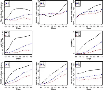
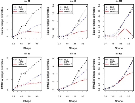
In what follows the aim is to compare the performances of the Maximum Marginalized order statistics Likelihood method (MMosLE) to that of the two alternative methods outlined in the preceding subsection by using graphical displays of the statistics computed from Monte Carlo simulations.
First of all one notices that for the three methods under comparison the bias of the shape parameter’s estimate is positive. This means that all the three methods overestimate the shape parameter. The magnitude of the bias are comparable for the three methods for values of the shape parameter not greater than 1. The graphics above suggest also that the bias improves quicker as the sample size increases for the MMosLE method proposed in this paper. The RMSE of the shape estimator provided by the proposed method is smaller than that of the LSPF-MLE and BL methods when the actual value of the shape parameter is greater than 2.0; this suggests that the proposed estimator exhibits less variability amongst samples.
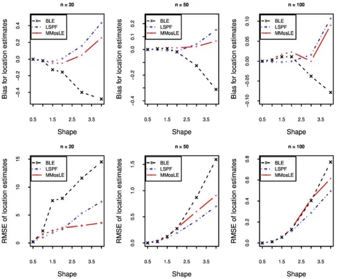
When sample is small the proposed method overestimates the location parameter as the LSPF-MLE method while the BL method underestimates the location. The magnitude of the bias of the proposed method is the smaller for value of the shape parameter larger than 1.5. When the sample size increases the magnitude of the bias of the estimator of the location parameter is comparable for the proposed method and the LSPF-MLE method. Both methods overestimate the location parameter as the actual value of the shape parameter increases (larger than 2.0). The graphics suggest also the magnitude of the RMSE is comparable between the LSPF-MLE method and the method proposed in this paper and outperform the BL method.
Figure 8. Bias and RMSE for scale parameter estimates based on 1000 simulated samples.
The bias of the scale parameter’s estimator has a magnitude larger than that of the LSPF-MLE estimator and the BL estimator. This bias is positive for the three estimators and increases with the magnitude of the shape parameter. Nevertheless the magnitudes of root-mean-squared-errors are
comparable for MMosLE method and the LSPF-MLE method or smaller. The root mean-squared-errors of the parameters’ estimators increase as the shape parameter increases for the three alternative methods but they improve as the sample size increases.
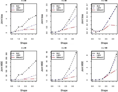
As one might be expected, the joint bias and joint MSE generally increase with the shape parameter for all the three methods. However the magnitude of both statistics decreases as the sample size increases. When the theorical value of the shape parameter is less than 1.0, the joint bias and joint MSE of the three methods are comparable. In other cases, the MMosLE method outperforms other methods, based on joint bias and joint MSE.
5. Illustrative Example: Maximum Flood
Dataset
Practical application of the proposed method is considered in this section by fitting the three-parameter gamma distribution to the well known dataset on maximum flood levels from Antle and Dumonceaux (1973) [19]. This dataset gathers the records of the maximum flood levels in millions of cubic feet per second for the Susquehanna River at Harrisburg, Pennsylvania, over 20 four-year periods from 1890–1969. Several authors, including Hirose (1995), Nagatsuka & al. (2014), Hall and Wang (2005), ([20, 3, 10]), have considered this dataset in the past to illustrate the efficiency of estimation methods for three-parameter gamma model, althought Antle and Dumonceaux did not initially consider this dataset for an estimation method effectiveness study. The estimates obtained by using the MMosLE method proposed in this paper is discussed hereafter with those obtained using the LSPF-MLE and BL methods respectively.
5.1. Parameters’ Estimates Using MMosLE Method and LSPF-MLE and BL Methods
The table below displays the estimates of the model’s parameters using three alternative methods: the Maximum Marginalized order statistics Likelihood (MMosLE) that motivates this paper, the Location and Shape Parameters Free-Maximum likelihood (LSPF-MLE) introduced by Nagatsuka & al. (2014), [3] and Bayesian Likelihood proposed by Hall and Wang (2005), [10]. Estimates obtained with MMosLE method are followed by an estimated bootstrap bias and a bootstrap 95% − confidence interval. Estimates obtained with LSPF-MLE method and BL method are reported from Nagatsuka & al. (2014), [3].
Table 4. Dumonceaux and Antle dataset: parameters’ estimates using MMosLE, LSPF-MLE and BL methods. (estimates obtained by LSPF-MLE and BL are reported from Nagatsuka & al. (2014)).
Shape Location Scale MMosLE 3.020 0.208 0.071 LSPF-MLE 2.371 0.235 0.080 BL 1.986 0.244 0.090
All the three methods give positive estimates of the location parameter. Substantial differences in the magnitude of the shape parameter’s estimates should be noticed: the MMosLE method gives the largest estimate of the shape
parameter and the smallest estimate is given by the BL method. Further, smallest estimates of the location and the scale is obtained with the MMosLE method while the BL method gives the largest estimate.
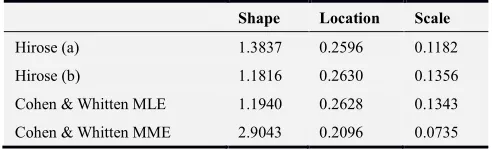
Several other earlier papers dealing with the fitting of the three-parameter gamma distribution, including Cohen and Whitten (1982), Hirose (1995), Tzavelas (2009)([2, 20, 11]), have resorted to this dataset to illustrate the behavior of their estimating methods. In the framework of the likelihood maximization, Hirose (1995) [20] and Tzavelas (2009) [11] found by different approaches that the log-likelihood has a local maximum reported in the second line of Table 5 (labelled ’Hirose (a)’). Hirose pointed out that the log-likelihood has a saddle point reported in the third line in Table 5 (labelled ‘Hirose (b)’) and this was confirmed by Tzavelas [11]. This saddle point appears to be very close to the model’s parameters estimates obtained by Cohen and Whitten (1982), [2], using maximum likelihood method (fourth line in Table 5. Their modified Moment Estimate method (MME) gave estimated values that are close that obtained by MMosLE procedure, Cohen and Whitten (1986), [21]. This exemple suggests that for samples of small size the maximum likelihood estimates may exhibit significant differences with estimates provided by other estimating procedures.
Table 5. Three-parameter gamma model fitted on Dumoceaux & Antle dataset.
Shape Location Scale Hirose (a) 1.3837 0.2596 0.1182
Hirose (b) 1.1816 0.2630 0.1356
Cohen & Whitten MLE 1.1940 0.2628 0.1343
Cohen & Whitten MME 2.9043 0.2096 0.0735
5.2. Diagnostic Plots for Goodness-of-Fit
Figure 10. Goodness-of-fit diagnostic plots.
Note that this dataset was not originally used by Dumonceaux & Antle (1973) in [19] for probability distribution fitting purpose; their aim in using this dataset was to illustrate the claim that “the ratio of maximized likelihood provides a good test for selecting” one distribution between the log-normal and the Weibull distributions.
5.3. Bootstrap Estimates of the Bias and the Confidence Interval Using MMosLE Method
The bias and the confidence intervals are computed by using the parametric bootstrap approach (Carpenter and Bithell (2000), [22]). 5000 samples of size 20 from the three-parameter gamma distribution are generated with the parameters equal to the fitted values.
One observes first that the confidence interval for the shape parameter is broad. The confidence interval of the location parameter includes zero as possible value for this parameter. The confidence intervals for the shape parameter and the scale parameter include no negative values.
Table 6. Bootstrap estimates of bias and bias-corrected percentile 95%-confidence interval.
Shape Location Scale Bias 5.301 -0.046 0.005 95% CI’s lower bound 1.014 -0.447 0.012 95% CI’s upper bound 64.582 0.282 0.174
6. Conclusion
In this paper maximum likelihood approach is proposed to estimate the parameters of the three-parameters gamma distribution. The likelihood is based on n − 1 largest order statistics of a sample of size n from a three-parameter gamma distribution. The maximum likelihood estimates of the model’s parameter is obtained under the constrain that the location parameter is larger than the first order statistics and by resorting to a MM-algorithm by doing like that all the dataset is taken into account in the estimation procedure. Although the distributions of the estimates exhibit skewness
when sample size is small or medium, the results of Monte Carlo simulation study suggest that the method is efficient as the bias and the root-mean-square error improve as the sample size increases. These results are compared with those of two alternative methods: the location and scale parameters free maximum likelihood estimators (LSPF-MLE) method of Nagatsuka & al. (2014), and the Bayesian Likelihood (BL) method of Hall and Wang (2005). The main conclusions of that comparison are as follows
(1) The bias of the shape parameter has a small magnitude when its actual value is less than 1.5 and it improves quicker than for LSPF-MLE and BL in all the domain of this parameter. The RMSE of the shape parameter estimate improves quicker than for LSPF-MLE and BL.
(2) The bias of the location parameter is small if the actual value of the shape parameter is less than 1.5 and its magnitude is comparable to the case of LSPF-MLE and BL if the actual value of the shape parameter is greater than 1.5.
The RMSE of the LSPF-MLE is the smallest of the three methods but the RMSE of the BL method is the worse with respect to this performance metric
(3) The scale parameter estimate computed by the LSPF-MLE method or the BL method has smaller bias than the MMosLE method.
The RMSE has a magnitude close to that of LSPF-MLE.
7. Appendix
7.1. Some Basic Inequalities
Let u, v, u′ and v′ be strictly positive real numbers. The following assertions hold
1. −79: | ≥ −79: |′ | |′ |′⁄
2. #| E #-|′ 2#′⁄ |-#′ 2|′⁄
3. 79: # = | E
79: # = |′ = |′79: | |⁄ ′ # = |′⁄
As a consequence of the inequalities (7.1) stated above one has
-since
79: | = 79: K1|L E 79: |′ −|′| − 1
7.2. Proof of Proposition 3.1
7.2.1. Minorizing the Terms in the Expression ~• €|•‚:ƒ, ⋯ , •ƒ:ƒ
79: ?: − ≥ 79: ?: − ′ + j : − ′ ?: − ′k
− j : − ′ ?: − ′k
-2 ′ − ?: : − ′− ′
: − ′ -: −
-′ 2
Since 79: ?: − = 79: ?: − : + : − ,
the basic inequality (7.1) leads to
79: ?: − ≥ 79: ?: − ′ + : − ′ ?: − ′ 79:
: − : − ′
Thus
79: ?: − ≥ 79: ?: − ′
+ : − ′
?: − ′ 79: : − : − ′
Applying inequality (7.1) and taking into account that λ>0 and one has
79: ?: − ≥ 79: ?: − ′ + j : − ′ ?: − ′k
− j : − ′ ?: − ′k
-2 ′ − j ?: : − ′− ′k
: − ′ -: −
-′ 2
−79: ?: − ≥ −79: ?: − ′ + − ′
?: − ′
− 79: ≥ − 79: ′ + −2 ′ − ′- 2 ′-
-7.3. Proof of Proposition 3.2
1. By applying the convexity inequality to the − log function one obtains
−79: ?: − ≥ −79: ?: − ′ + − ′
?: − ′
Moreover
− 79: ≥ j−79: ′ − − ′′ k
≥ − 79: ′ + − 1′ j2- ′ +′ 2- ′′k
≥ − 79: ′ + −2 ′ −- 2 ′′ -
-2. One has
„ = " #
@ −
1;
-: − #<%#
and by Jensen inequality one obtains
7- | -: , ⋯ , : ≥ 79:;R@ ′ < + − ′ R ′
− …1 -: − − 1′ -: − ′ † R- ′
Applying the basic inequality (7.1) results in what follows:
−1 -: − ≥ − ′ -: 2 -− ′ − -: − -2 ′ -: − ′
and thus
7- | -: , ⋯ , : ≥ 79:;R@ ′ < + − ′ R ′
− ′ -: 2 -− ′ R- ′ −R- ′ -: − -2 ′ -: − ′ +R- ′ -: − ′
′
References
[1] B. and Ashkar Bobee: The gamma family and derived distributions applied in hydrology. Water Resources Publications, 1991.
[2] A. C Cohen, B. J. Whiten: “Modified moment and maximum likelihood estimators for parameters of the three-parameter gamma distribution”, Communications in statistics-simulation and computation, pp. 197-216, 1982.
[3] H. Nagatsuka, N. Balakrishnan, T. Kamakura: “A consistent Method of Estimation For the Three-Parameter Gamma Distribution”, Communications in Statistics-Theory and Methods, pp. 3905-3926, 2014.
[4] K. O. and Shenton Bowman: “Problems with maximum likelihood estimation and the 3 parameter gamma distribution”, Journal of Statistical Computation and Simulation, pp. 391-401, 2002. [5] R. C. H. Cheng, T. C. Iles: “Embedded models in three-parameter
distributions and their estimation”, Journal of the Royal Statistical Society. Series B (Methodological), pp. 135-149, 1990.
[6] R. C. H. and Iles Cheng: “Corrected maximum likelihood in non-regular problems”, Journal of the Royal Statistical Society. Series B (Methodological), pp. 95-101, 1987. [7] R. L. Smith: “Maximum likelihood estimation in a class of
nonregular cases”, Biometrika, pp. 67-90, 1985.
[8] G. Tzavelas: “Sufficient conditions for the existence of a solution for the log-likelihood equations in three-parameter gamma distribution”, Communications in Statistics-theory and methods, pp. 1371-1382, 2008.
[10] P. Hall, J. Z. Wang: “Bayesian Likelihood Methods for estimating the end point of a Distribution”, Journal of the Royal Statistical Society, pp. 717-729, 2005.
[11] G. Tzavelas: “Maximum likelihood parameter estimation in the three-parameter gamma distribution with use of Mathematica”, Journal of Statistical Computation and Simulation, pp. 1457-1466, 2009.
[12] K. and Hunter Lange, I. Yang: “Optimization transfer using surrogate objective functions (with discussion)”, Journal of Computational and Graphical Statistics, pp. 1-20, 2000. [13] D. R. Hunter, K. Lange: “A tutorial on MM algorithms”, The
American Statistician, pp. 30-37, 2004.
[14] K. Lange: Optimization, Second Edition. Springer New York, 2013.
[15] W. C. F. Jeff: “On the Convergence Properties of the EM Algorithm”, The Annals of Statistics, pp. 95-103, 1983. [16] F. Vaida: “Parameter convergence for EM and MM
algorithms”, Statist. Sinica, pp. 831-840, 2005.
[17] R Core Team: R: A Language and Environment for Statistical Computing. http://www.R-project.org/, 2015.
[18] M. Becker, S. Klößner: PearsonDS: Pearson Distribution System.. http://CRAN.R-project.org/package=PearsonDS, R package version 0.97, 2013.
[19] R. Dumonceaux, C. E. Antle: “Discriminations between the log-normal and the weibull distributions”, Technometrics, pp. 923-926, 1973.
[20] H. Hirose: “Maximum likelihood parameter estimation in the three-parameter gamma distribution”, Computational Statistics and Data Analysis, pp. 343-354, 1995.
[21] A. C. Cohen, B. J. Whitten: “Modified moment estimation for the three-parameter gamma distribution”, Journal of Quality Technology, pp. 53-62, 1986.