http://www.sciencepublishinggroup.com/j/ajam doi: 10.11648/j.ajam.20180602.11
ISSN: 2330-0043 (Print); ISSN: 2330-006X (Online)
An Adjusted Trinomial Lattice for Pricing Arithmetic
Average Based Asian Option
Dennis Odhiambo Ogot, Phillip Ngare, Joseph Mung’atu
Mathematics, Pan African University Institute for Basic Sciences, Technology and Innovation, Nairobi, Kenya
Email address:
To cite this article:
Dennis Odhiambo Ogot, Phillip Ngare, Joseph Mung’atu. An Adjusted Trinomial Lattice for Pricing Arithmetic Average Based Asian Option.
American Journal of Applied Mathematics. Vol. 6, No. 2, 2018, pp. 28-33. doi: 10.11648/j.ajam.20180602.11 Received: November 9, 2017; Accepted: November 22, 2017; Published: March 24, 2018
Abstract:
An adjusted trinomial model for pricing both European and American arithmetic average-based Asian options is proposed. The Kamrad and Ritchken trinomial tree governs the underlying asset evolution. The algorithm selects a subset of the true averages realized at each node to serve as the representative averages. The option prices are then computed via backward induction and interpolation. The results show that the trinomial method produces more accurate prices especially in the case of European style Asian options.Keywords:
Asian Options, Arithmetic Average, Lattice, Trinomial1. Introduction
An Asian option is an exotic path dependent option. Its value is pegged on the average underlying asset’s price over the option’s life. The averaging feature makes them attractive as they are less prone to market manipulation at maturity. This also results in them being cheaper than plain European or American options.
Usually the averages that are considered are the arithmetic and geometric average. The latter is straight forward as it results in a closed form expression for European options in line with the classical Black Scholes model [1]. This is because geometric average follows the same lognormal distribution as the underlying variable thus easing the mathematical tractability of the pricing problem. However, this is not the case for Asian options priced using the arithmetic average which does not follow a lognormal distribution. This is in spite of it being far more popular and widely used than its geometric average counterpart.
Due to its wide use there has been numerous attempts to tackle the pricing problem of arithmetic average options. Most of this models involve some forms of numerical approximations. A number of researchers used analytical approximation to price Asian options [2] [3], and approximate the arithmetic average with the corresponding geometric average. While this approaches are straight forward, their accuracy is found wanting in some cases. Turnbull and
Wakeman [4] use edge worth expansions to improve the approximations.
Early models used to solve the partial differential equations governing the option’s price encountered problems too. Wilmott et al [5] found stability issues when using the explicit finite difference method while the implicit finite difference method only works with certain volatility structures. Vecer [6] came up with a method that overcomes the stability of problems encountered before but like all the methods mentioned above it cannot work for American Asian options.
It is this shortcoming that among others make lattice based models more suited for pricing arithmetic average-based Asian options. They work not only for European Asian options but also for American style Asian options. They are also efficient, flexible, and simple to use. The challenge with using these models to price Asian options, is the enormous number of averages to be kept track of. They increase exponentially with an increase in the time steps used. This is because unlike the geometric average, the arithmetic average does not recombine in the lattice.
2. Lattice Based Models for Pricing Asian
Options
A lattice is made up of node and edges that connect them. It is used to simulate the price process of an asset. Suppose that an item is written at time t=0 and has time of maturity as t =T, the lattice divides the time interval equal time steps. This makes it a discrete approximation of what is the continuous price process of the underlying. The simplest of the lattice methods is the binomial tree method where it is assumed that at each time step the price of the underlying can only move either up or down.
Hull and White [7] outlined the first binomial lattice model to price arithmetic average-based Asian options. They consider a European Asian call option. Their model is based on the well-known CRR binomial tree advanced by [8]. The underlying’s price either grows by a factor of u or lessens by a factor d with a probability of and at any time step where:
= exp ( √∆ ) and = (1)
= ( ∆ = 1 − (2)
Let ( , ! represent the price of the underlying at node
( , ! denoting the node arrived at after j upward moves followed by ( − ! downward moves have occurred. To combat the huge number of non-recombining averages they simulated a smaller set of averages to represent the enourmous amount of averages realized at each increasing time step [7]. The maximum and minimum averages at time step ∆ , denoted "#$%( and "#&'( take the form of ()±#+. Here, h takes a constant value whereas m represents the least integer satisfying the following equations:
",-.( = ) #+≤$0 1 "#$%(i − 1 + 4 − 1,067 (3)
"#&'( = ) #+ ≥$0 1 "#&'( − 1 + 4 − 1, ! − 167 (4)
The other averages at that time step take the form
()9+where : takes the value of all integers from – (< − 1
to (< − 1 . If " ( , !, : is the :+ average for a particular time step, the value of the option denoted =( , !, : associated with it is then computed by discounting the payoffs form the next time step (backward induction) i.e.
=( , !, : = ) ∆ ( =4 + 1, ! + 1, : 6 + =4 + 1, !, : 6 (5)
Where =4 + 1, ! + 1, : 6 and =4 + 1, !, : 6 correspond to
" =4($0 > ($,?,9 0 @($,? 6($0A (6)
and
" =4($0 > ($,?,9 0 @($,? 6($0A (7)
=4 + 1, ! + 1, : 6is then further approximated since its exact value is usually not in the set of representative averages. Linear interpolation is done using the averages present that are
closest to " and " . The same is done for =4 + 1, !, : 6. One challenge with this method is that there is no standard way of coming up with parameter h which affects how many representative averages will be simulated at each time step. The option prices calculated are actually indirectly proportional to the value of h. This is due to the linear interpolation which overestimates the price. Another weakness stems from the fact once h is chosen, the price of the option is directly proportional to the number of time steps used in the tree.
Forsyth et al [9] improved on the model by choosing h to be directly proportional to the size of a time step ∆ so as to bring about convergence. Thus their results are more stable than those of Hull and White. They set
ℎ = αEF.AGH A∆ (8)
They however do not prescribe how to choose the values of other parameters.
Costabile et al [10] came up with a highly efficient model based on Hull and White. Their key improvement on the previous models is that they choose a subset of the actual averages at a node unlike in the earlier methods where the averages are simulated. At the node (i, j) of the binomial lattice, they first calculate the highest average "#&' ( , ! which is the result the price path I#&'( , ! denoting the path starting j up moves followed by( − ! down moves. The last element of the set at each node is the lowest average
"#$%( , ! resulting from I#$%( , ! , the path starting with
( − ! down moves followed by j up moves. The remaining averages are computed recursively as follows. If #&'( , !, : denotes the highest underlying asset price realized in the price path producing " ( , !, : (the kth average) that is not in the trajectory I min( , ! then:
" ( , !, : + 1 = " ( , !, : −L0 4 #&'( , !, : − #&'( , !, : A6 (9)
This is repeated until the path I#$%( , ! is reached. Once the representatives are obtained, the same backward induction described earlier is used to calculate the option’s price.
One advantage of this method [10] is that there are no other parameters that need to be computed beforehand. This would have led to the issues encountered in the earlier methods. Also, the number of times linear interpolation is required is greatly reduced as the set of averages considered are a subset of the true realized averages at a particular node. This means that more often than not the average required will be found in the next time step. In this paper, the aim is to extend this concept to a trinomial lattice to see how much better the prices computed will be.
Zvan et al [11] proposes a numerical scheme to price American style Asian options using the Crank –Nicolson method. Klaasen [12] sets out a binomial method using 512 time steps to price American Asian options. Instead of linear interpolation, he applies Richardson extrapolation to hasten convergence.
underlying price at every node to be a rational number of finite precision. It is partitioned into different parts with varying resolution hence reducing the number of averages considered. It is based on the premise that if the underlying asset prices are multiplied by a constant before pricing the option, then option value divided by the same constant gives the originally desired option value. Convergence is ensured by making sure the underlying asset’s price process simulated mirrors to the continuous time lognormal price process of the underlying. Their work shows that this method converges as the time steps used are increased. In the next section the proposed trinomial model is laid out in more detail.
3. Proposed Trinomial Algorithm
The trinomial model allows for us to model a case where the asset price now moves on of three ways, up, down or stay in the middle. The Kamrad and Ritchken [15] tree matches the 1st moment and variance in the log space. The asset may increase by a factor of
= expMN √∆ O (10)
It may decrease by = . Additionally it may remain at the same level i.e. multiplied by < = 1. N is an important Parameter as if not chosen appropriately, the values of the probabilities of an up move , down move and staying at the same price, # may be negative. Boyle [14], found that the price are most accurate when all the probabilities are roughly equal. Kamrad and Ritchken [15] make this possible by choosing:
N = 1.22474 (11)
=AST+U√∆ASV (12)
=AST−U√∆ASV (13)
and
# = 1 − − (14)
The numeral results in this paper were computed using an adjusted trinomial model based on the Kamrad and Ritchken trinomial tree.
The modified trinomial method for pricing Arithmetic average based Asian option is an extension of the one used by Costabile et al. The modification made is based the method of choosing representative averages in order to carter for the ‘’middle’’ moves in the trinomial tree that were not in the binomial tree. Let $,? denote the ! + node at the + time step. The number of up, middle and down jumps are defined as W ,W# and W respectively. Therefore the value of the underlying at node j of time step is
$,?= XY XZ (F,F [ℎ)\) W + W#+ W = (15)
First, the path I$,?#&' which results in the highest average at a particular node denoted by "$,?#&' is considered. I$,?#&'is now the price path constituted by W up steps followed by
W# middle steps and then W down steps to get to $,? . "$,?#&'
is the first representative average at that particular node denoted "( , !, 1 . The :+ average "( , !, : is then recursively calculated using the previous average. The first highest average denoted #&'( , !: : − 1 realized on the previous price path is replaced by #&'( , !: : − 1 . This is repeated till the minimum average possible at the particular node is reached. This is the average associated with the price path I$,?#$%. This is the path made by W down steps followed by W# middle steps and then W up steps to get to $,? .
Once all the averages at the time step are obtained, the payoffs corresponding to the averages are computed. Then the option price are computed using the usual induction scheme that is;
=$? 9 = ) ∆ 4 =$0 ,?9Y + #=$0 ,?09^ + =$0 ,?0A9^ 6 (16)
In some cases, =$0 ,?_ , =$0 ,?0_# =$0 ,?0A_ are computed via linear interpolation. For American Asian options where early exercise is allowed the value of the option at $,? is:
=$,?9 = maxa) ∆ a =$0 ,?9Y + #=$0 ,?09^ + =$0 ,?0A9^ b, $,?9 − :b (17)
The model shares the same advantages as the binomial one by Costabile et al. Since the representative averages are a subset of the true realized averages, the instances where interpolation is required are greatly reduced. In fact they are even lesser in this case as more averages are computed than in the binomial case.
4. Results
The results that were computed through the trinomial algorithm for both European and American style Asian Options are now presented.
4.1. European Asian Options
Table 1. European call option values using the trinomial algorithm, the method by Costabile et al and the multiresolution trinomial lattice by Dai.
TIME STEPS K=40 K=50 K=60
Costabile Trinomial Costabile Trinomial Costabile Trinomial
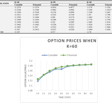
10 11.5276 11.5274 4.5014 4.4877 1.1176 1.1258
15 11.5348 11.5346 4.5082 4.4992 1.1428 1.14327
20 11.5384 11.5364 4.5126 4.5094 1.1548 1.1601
30 11.5413 11.5427 4.5165 4.5149 1.167 1.1706
40 11.5302 11.5446 4.509 4.5176 1.1665 1.1761
50 11.5449 11.5454 4.5209 4.5192 1.1778 1.1794
60 11.5458 11.5463 4.522 4.5205 1.1805 1.1818
70 11.5463 11.5463 4.5228 4.5213 1.1824 1.1834
80 11.5467 11.547 4.5233 4.5221 1.1838 1.1846
90 11.547 11.5472 4.5237 4.5226 1.1849 1.1856
Dai MR 11.547 4.517 1.170
Figure 1. European Asian option values from the trinomial method and the algorithm by Costabile et al when the exercise price K = 60.
4.2. American Asian Options
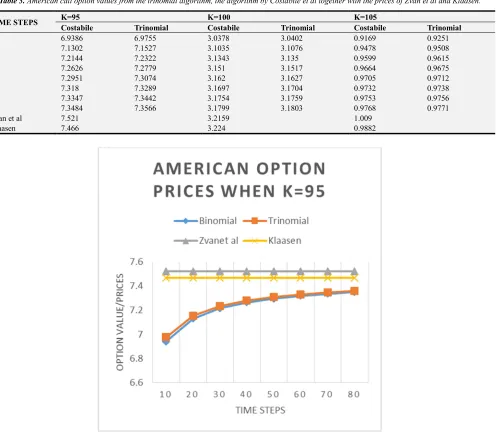
The results for American style options are compared by with the algorithms by [10], [11] and [12]. The option whose prices are in Table 2 were written on an underlying with initial price of 50, time to maturity of 1 year, a volatility of 30%, a risk free interest rate of 10% and various exercise prices K. Again the trinomial model only slightly
outperforms the model by [10]. Table 3 shows option values written on an underlying with an initial price of 100, time to maturity of 0.25 years, volatility of 20% and a risk free rate of 10%. The prices by [11] and [12] are used as the “true” option values. As illustrated in figure 2, the prices by the trinomial algorithm do not significantly outperform the algorithm by [10] in pace of convergence or smoothness
Table 2. American call option values from the trinomial algorithm, the algorithm by Costabile et al.
TIME STEPS K=40 K=50 K=60
Costabile Trinomial Costabile Trinomial Costabile Trinomial
10 12.6824 12.6842 4.7097 4.6974 1.1279 1.1376
20 12.9562 12.9721 4.8134 4.8172 1.1772 1.1834
30 13.0756 13.0987 4.8619 4.8621 1.1951 1.1992
40 13.1416 13.1678 4.8793 4.8885 1.1975 1.2077
50 13.1986 13.2159 4.9053 4.9058 1.211 1.2131
60 13.2347 13.2508 4.9175 4.9181 1.2152 1.2168
70 13.2612 13.2747 4.9264 4.9268 1.2181 1.2194
Table 3. American call option values from the trinomial algorithm, the algorithm by Costabile et al together with the prices of Zvan et al and Klaasen.
TIME STEPS K=95 K=100 K=105
Costabile Trinomial Costabile Trinomial Costabile Trinomial
10 6.9386 6.9755 3.0378 3.0402 0.9169 0.9251
20 7.1302 7.1527 3.1035 3.1076 0.9478 0.9508
30 7.2144 7.2322 3.1343 3.135 0.9599 0.9615
40 7.2626 7.2779 3.151 3.1517 0.9664 0.9675
50 7.2951 7.3074 3.162 3.1627 0.9705 0.9712
60 7.318 7.3289 3.1697 3.1704 0.9732 0.9738
70 7.3347 7.3442 3.1754 3.1759 0.9753 0.9756
80 7.3484 7.3566 3.1799 3.1803 0.9768 0.9771
Zvan et al 7.521 3.2159 1.009
Klaasen 7.466 3.224 0.9882
Figure 2. American Asian option prices for the trinomial algorithm and the binomial method by Costabile et al compared to those of Zvan et al and Klaasen.
5. Conclusions
The binomial algorithm for Asian options by (10) is extended to a trinomial setting using the lattice proposed by (15). A subset of the true averages realized at each node are considered as the representative averages for use. The algorithm is tested for both European and American style Asian options. It is simple to use and very flexible. The results show it gives more accurate option values with an especially smoother convergence than the previous models.
References
[1] Zhang, P. G. Exotic Options: A guide to second generation options. s. l.: World Scientific, 1998.
[2] Pricing European Average rate currency options. Levy, E. 1992, International Money and Finance, Vol. 11, pp. 474-491.
[3] Prices and Hedge ratios of Average rate exchange options.
Vorst, T. 1992, International Review of Financial analysis, Vol. 1, pp. 179-193.
[4] A quickalgorithm for pricing European average options. S. M. Turnbull, L. M. Wakeman. 3, 1991, Journal of Financial and Quantitative Analysis377-389, Vol. 26.
[5] P. Wilmott, J. Dewynne, S. Howison. Option Pricing: MAthematical Models and Computation. Oxford: Oxford Financial Press, 1993.
[6] A new PDE approach for pricing arithmetic average Asian options. Vecer, J. 4, Journal of Computational Finance, Vol. 4, pp. 105-113.
[7] Efficient Procedures for valuing European and American path-dependent options. J. Hull, A. White. 1993, Journal of Derivatives, Vol. 1, pp. 21-31.
[9] Convergence of Numerical Methods for Valuing Path Dependent Options using Interpolation. P. A. Forsyth, K. R. Vetzal and R. Zvan. 2002, Rev Derivatives, Vol. 5.
[10] An adfjusted binomial model for pricing Asian options. M. Costabile, E. Russo and I. Massabo. 2006, Rev Quant Finance, Vol. 27, pp. 285-296.
[11] Robust Numerical PDE models for Asian Options. R. Zvan, P. A. Forsyth and K. R. Petal. 2, 1998, Journal of Computational Finance, Vol. 1, pp. 39-78.
[12] Simple, Fast and Flexible pricing of Asian options. Klaasen, T. R. 3, 2001, Vol. 4, pp. 89-124.
[13] Pricing Asian options with Lattices. Dai, T. S. s. l.: Department of Computer Science and Information Engineering, National Taiwan University, 2004, Ph.D. Thesis.
[14] Option valuation using a three-jump process. Boyle, P. 7-12, 1986, International Options Journal, Vol. 3.