http://www.sciencepublishinggroup.com/j/ajam doi: 10.11648/j.ajam.20180603.12
ISSN: 2330-0043 (Print); ISSN: 2330-006X (Online)
Modeling and Simulation Study of Mutuality Interactions
with Type II functional Response and Harvesting
Solomon Tolcha
1, Boka Kumsa
1, Purnachandra Rao Koya
21
Department of Mathematics, Wollega University, Nekemte, Ethiopia
2Department of Mathematics, Hawassa University, Hawassa, Ethiopia
Email address:
To cite this article:
Solomon Tolcha, Boka Kumsa, Purnachandra Rao Koya. Modeling and Simulation Study of Mutuality Interactions with Type II functional Response and Harvesting. American Journal of Applied Mathematics. Vol. 6, No. 3, 2018, pp. 109-116.
doi: 10.11648/j.ajam.20180603.12
Received: May 25, 2018; Accepted: June 26, 2018; Published: July 31, 2018
Abstract:
This paper deals with the study of mutuality interactions between two species population with type II functional response and also with the inclusion of harvesting. Harvesting functions are introduced to express the rate of reductions of the species separately. Mathematical model have been constructed and considered for the analysis and results. In this model, the first population species benefited according to type II functional response and the second species benefited from the first according to type I functional response and also harvested proportional to its density. It is shown that the model has positive and bounded solutions. Stability analysis is carried out. The local and global stability of biologically interested equilibrium point are considered and analyzed. Numerical examples supporting theoretical results such as phase plane and simulation study using DSolver are also included. Assumptions and results are presented and discussed lucidly in the text of the paper.Keywords: Mutualism, Functional Response, Harvesting, Phase Plane Analysis, Positivity and Boundedness
1. Introduction
Mutualism is the way where populations of two different species exist and live in some relationship in which each individual benefits from the activity of the other [1]. In case of mutualism both the species experience increment in their population sizes. However, mutualism has historically received less attention than other interactions such as predation, competition and parasitism [2, 3].
Mutualism can be categorized according to the way of dependency of one species on the other. Accordingly, mutualism can be divided into two broad categories viz., obligate mutualism and facultative mutualism. Obligate mutualism is a type of mutualism in which the species interdependent with one another in a way that one cannot survive without the other. Facultative mutualism can be defined as a type of mutualism in which the interacting species receive benefit from each other but are not fully dependent. However, the facultative is the most common mutualism in ecology. Some common examples of facultative mutualism are (i) zebra and wildebeest and (ii) plants
producing fruit that is eaten by birds and the birds helping to dispose the seeds through excretion [4].
A good example of mutualism interactions considered in this paper is the consumer – resource mutualism kind of interactions like prey – predator interaction. The difference is that in mutualism both species are benefited while in prey – predator system only the predator population is benefited. The consumer – resource interaction was originally incorporated into the study of inter specific interactions to provide a mechanism for the ways by which individuals interact with one another [5, 6]. The most common examples of consumer – resource interactions are pollinator and flowering plants in which pollinator are consumers and flowering plants are resources. Here, the pollinators obtain the flora nectar or pollen as a food resource while the plant obtains non – tropic reproductive benefits through pollen dispersal and seed production.
P. F. Verhulst modifies Robert Malthus’s equation and proposed logistic equation as [7]
In (1), it is assumed that the growth parameter decays linearly and becomes zero when environmental conditions are saturated and the population reaches its maximum value called carrying capacity . Here, is defined as the maximum population size that the environment can sustain indefinitely in the given conditions of water, nutrients and other necessities.
The classical Lotka –Volterra model is modified by assuming that both the mutualistic interacting species grow following logistic function with the inclusion of a positive or beneficial interaction term proportional to both populations as given in [8] as
⁄ = 1 − ⁄ + (2)
⁄ = 1 − ⁄ + (3)
Here in (2) and (3), all the parameters , , , , and are considered to be positive constants. However, the helping rate of both populations is unlimited. That is, as the density of the first population increases the helping rate received by the first population from the second population also increases and vice versa. But, in practice this may not always be true.
The controlled mutualistic model given by (2) and (3) was proposed by [9]. In that study the Lotka –Volterra equations were modified by adding new term to represent a mutualistic relationship. The study also considered the concept of saturation i.e. in mutualistic interactions, as the densities of population grow higher the benefits received from the mutualistic population is decreased. If the saturation concept is neglected then the species abundance or density of population would be expected to increase indefinitely. However, it is not possible to neglect saturation due to environmental factors and carrying capacities of populations. Hence, a model that includes saturation would be more realistic for large populations.
The most accepted model for mutualistic communities or populations with limited growth is called Type II functional response. A two – species model is proposed with limiting mutualistic term as a Type II functional response that includes the effect of handling time [9].
The other method called harvesting which is used to control growth of species. The process of harvesting is frequently used to exploit biological species so as to meet the needs of human beings and the society [10]. Different types of harvesting functions have been used in mathematical modeling [11 – 15].
The most important harvesting strategy is catch – per – unit – effort. In a mathematical modeling this concept is represented by a harvesting function = q E N t . Here, is the catchability coefficient; is the constant external effort; and is the density of the harvested species. The Catch – per – unit – effort based harvesting has been widely accepted and believed to be the more realistic than its constant harvesting counter part because the former is proportional to the density of the harvested species [16].
The harvesting management in general considers mainly two important purposes: (i) to control the increase of a
species population and (ii) to meet the demands of human society [17].
Some works from literature are considered and extended with the inclusion of some reasonable assumptions. The existing model of mutualistic interactions of two species populations is briefly introduced. Then a new model has been proposed and developed to explain the dynamical behavior of interaction over the existing model. The currently proposed model modifies the existing model so as to correctly address a realistic situation.
The existing mutualistic interaction model of two species population in which both population are benefited from each other according to type I functional response or linear way and both populations are harvested with density dependent function or proportionally harvested can be expressed by the following system of equations [18]:
⁄ = 1 − ⁄ + − ℎ (4) ⁄ = ! 1 − ⁄ " + # − ℎ$ (5) Here in (4) to (5), various variables and parameters are used to represent the following: (i) the variables and denote the population sizes of first and the second species respectively at time (ii) and ! are the respective intrinsic growth rates (iii) and $ are respective carrying capacities (iv) and # are the mutualism effect of on and on respectively (v) ℎ and ℎ$ are the harvesting terms proportional to the respective population sizes. Moreover, all the parameters are assumed to be positive constants.
2. Governing Equations of the Model
In this section, the existing model described by the equations (4) – (5) is modified with the inclusion of two assumptions: (i) the benefit received by the first population from the second population is according to type II functional response and (ii) also in place of harvesting both populations at the same time, in this new model the second population alone is subjected to harvesting.
Thus, the mathematical model for the modified mutualistic interaction can be represented by a system of two equations as follows:
%&'
%( = )1 −
&' *'+ + ,
-'.&'&.
/-'.0&'1 (6) %&.
%( = )1 −
&.
*.+ + − (7)
Here in (6) and (7), the variables 2 and 2 denote respectively the densities of the first and the second species at any instant of time 2 subjected to the non – negative initial
conditions 0 = 4≥ 0 and 0 = 4≥ 0 . The
Additionally, the following assumptions have also been incorporated in order to construct the modified model given by (6) – (7).
(i) Both populations and grow logistically in the absence of interactions between the two species. Here, it is assumed that the species and do not grow indefinitely even in the absence of interactions with each other due to intra specific competition within each population. However, both the populations will grow and reach their respective maximum carrying capacities.
(ii) There exists a mutualistic relationship between and . That is, both the species are benefited from their interactions. Accordingly, the population helps according to type – I functional response or in a linear way. Which implies that for an infinitely large , the helping rate of too becomes infinite. In this case, the amount of help received by from a single per unit of time is referred to as – functional response and represented as . (iii) The population helps according to type – II
functional response. The type II functional response is based on the assumption that becomes saturated for large values of abundance i.e., the population becomes limited by their handling time at very
high densities of which is represented
as ) /--'.&' '.0&'+.
(iv) The second population is harvested with density dependent function or proportionally harvested.
2.1. Non – Dimensionalization of the Model
The main objectives for scaling the model equations are (i) to reduce the number of model parameters (ii) to make both model variables and parameters unit less and (iii) to make the model simple so as to conduct mathematical analysis easily.
To obtain the scaled form of the model equations (6) and (7), let the following transformation equations be considered:
= , = and 2 = 1⁄ . The quantities ,
and have no dimensions. Then, after substituting these new parameters and performing some algebraic manipulations the scaled form of the system of equations (6) and (7) is obtained as follows:
%7
%8 = 1 − + ) 9'. $
/:' + (8) %;
%8 = < 1 − + − <= (9)
Here in (8) to (9), various notations represent the expressions as =-'.>*.
' , < = ℎ , < = >. >', = -.'*'
>' , and <== ?.@.
>' .
Now the model equations are scaled and the parameters are reduced. It can be observed that the original model equations have ten parameters while the scaled one has only five. Thus, the scaling procedure has a big impact on the reduction of number of parameters.
Now it is possible to analyze the model equations in a
simpler manner. At this stage it is quite appropriate to show that the solutions of scaled model equations are positive and bounded.
2.2. Positivity of the Solutions
Proposition1. All solutions A of the system of equations (8) and (9) with positive initial conditions 4, 4 are positive i. e., > 0, > 0, for all ≥ 0. Proof: Positivity of : Now, the equation (8) is %7%8 = ,1 − + )9'.$
/:' +1. Here and are the function of t. So by using variables separable method the solution of this equation can be found as = 4C D E )1 − x ! +48
9'.$ "
/:' "+ !. Here 4 is the density of the initial population at = 0 which is constant. Also for every time t, the exponential function C D E )1 − x ! + 9/:'.$ "
' "+ 8
4 ! is
positive. Therefore, the solution = 4C D E 1 − x ! +48 9'.$ "
/:' " ! of the model is positive for all t.
Positivity of : Similarly the solution of equation (9), %;
%8 = < − < + − <= is given as = 4C D E < − < ! +48 ! − <= ! where 4 is the initial population at = 0 and the exponential function is also positive for all t. Therefore, the solution =
4C D E < − < ! +48 ! − <= ! is always positive for all t.
Hence, from the above two conditions the solutions A of the model equation (8) and (9) are positive for all ≥ 0
2.3. Boundedness of the Solutions
Lemma 1. The equation (8) of the model leads to the inequality G⁄ ≤ 1 − x 1 − < if the condition < − > 0 is satisfied.
Proof: Now, the model equation (8) can be expressed as ⁄ = I 1 − 1 + < + ⁄ 1 + < J . But, since the denominator 1 + < is greater than 1, the foregoing equation takes and inequality form as ⁄ ≤
1 − 1 + < + = 1 + < − x 1 + < + = 1 + < − x − < + = 1 − x 1 − < − < − .
Therefore it can be concluded that ⁄ ≤ 1 − x 1 − < if < − > 0
Theorem 1: All solution of A of the system of model equations (8) and (9) together with initial condition 4, 4 are bounded with in a region K = I , : 0 ≤
≤ M:', 0 ≤ ≤ 1 + 9'. :. M:'J.
Proof: Boundedness of : The lemma 1, gives %%8 ≤ 1 − x 1 − < . So by using partial fraction method, the solution of is given as: ≤ / M:NOP
'NOP where c is a constant. After substituting the initial conditions it is given as Q = M R
solution converges to a positive quantity M: ' for all < < 1. This shows that the solution for is bounded from above for all ≥ 0.
Boundedness of : Similarly, the model equation (9) can be expressed as %$%8 ≤ < + − < . Making use
of the fact = M:
' the foregoing inequality can be integrated to obtain ≤ NOV.WX.' 'YV'/N:⁄ P:./9.'⁄ M:'
.OV.WX.' 'YV'⁄ P . Here Q is an arbitrary integral constant. On substituting the initial condition it can be obtained that Q = : $R
./9.'⁄ M:'M$R:.. Then, as → ∞ the limiting value of the solution
converges to Z1 +: 9.'
. M:' [ for all < < 1. This shows the solution for is bounded from above for all ≥ 0.
Therefore, all solutions of the model with positive initial values are bounded in the region R.
2.4. Existence of Equilibrium Points
In this section, the equilibrium points of the system are determined. This is achieved by equating the first order differentials of model variables (8) and (9) to zero. Thus, the following non-negative equilibrium points are obtained:
i. D 0, 0 , It is a trivial equilibrium point. Here both species are washed out.
ii.D 0, ∗ ,here ∗=:
. < − <= > 0 for < > <= iii.D= 1,0
iv.D] ∗, ∗ Coexistence equilibrium point.
Here, coordinates of the coexistence equilibrium point are
found to be ∗=9
.' <=+ <
∗− 1 > 0, ^_ ∗>
1 ` <=+ < ∗− 1 > 0 and ∗=9'. ∗− 1 1 + < ∗ > 0, ^_ ∗> 1, for A different from zero.
2.5. Qualitative Analysis of the Model
In solving mathematical system of equations, sometime it is difficult to obtain analytical solutions for both variables ∗, ∗ . But it is possible to solve them numerically.
The present modified model has four equilibrium points of D 0, 0 , D 0, ∗ where ∗=:
. < − <= , D= ∗, 0
where ∗= 1 and the coexistence equilibrium point
D] ∗, ∗ where ∗=9
.' <=+ <
∗− 1 and ∗=
9'.
∗− 1 1 + < ∗ . All the four equilibrium points are
physically valid and meaningful for all parameters.
2.6. Local Stability Analysis at Each Equilibrium Points
In this section, the local stability analysis at each equilibrium points of model equations (8) and (9) is conducted. In order to determine the local asymptotically stability at each equilibrium point, the community matrix of model (8) and (9) is needed to compute and the eigenvalues from the characteristics equation of the matrices are to be found. The sign of the real part of the eigenvalues of this
matrix evaluated at the given equilibrium points determines its stability. So by using the community matrix, the local stability of the model is determined in the following way:
The left hand side expressions of the model equations are considered as functions as
_ , = 1 − + 1 + < a , = < 1 − + − <= Also their first partial derivatives are computed as
bc
b = 1 − 2 + 9'.$ /:' . , bc b$= 9'. /:' , be
b = , and
be
b$= < − 2< + − <=
Now, the community matrix of the model is defined as
f = g bc b bc b$ be b be b$
h and can be constructed for the present model
as
f = i1 − 2 + 1 + < 1 + <
< − 2< + − <= j
Theorem 2: The trivial equilibrium point D 0,0 is unstable and the boundary equilibrium points D 0, ∗) and D= 1,0) are saddle points.
Proof: The equilibrium point D 0,0 is unstable which is trivial.
The community matrix at the equilibrium point D 0, ∗) is
given as 0, ∗ = k1 +
∗ 0
∗ <
=− < l. Now, on solving the characteristics equation of this matrix eigenvalues are found to be m = 1 + ∗and m = <=− < = − ,. It can be observed that m is always positive since and ∗ are positive. Here, m is negative since the proportional harvesting requires the relation < . That is, m is positive while m is negative. Thus, the equilibrium point D 0, ∗) is saddle point and is unstable in general.
Similarly, The community matrix at the equilibrium
point D= 1,0) is given by: f 1,0 = n−1
9'. /:' 0 < + − <=o
.
Here, from solving the characteristics equation of this matrix the eigenvalues are obtained as m = −1 < 0 and m = < +
− <=> 0. That is, here m is negative while m is positive. Therefore, the equilibrium point D=is saddle point and thus it is unstable.
Local stability analysis at t D]: In determining the dynamical behavior of the species at the coexistence equilibrium point, the community matrix at the given equilibrium point should be found. The equilibrium points are substituted only in the diagonal entries of the matrix and the other two off diagonal entries are left as they are. This procedure is adopted just to make the computations simpler. Thus, the community matrix can be expressed as
f ∗, ∗ = )
Here = /:∗
' ∗ < 1 − 2
∗ − 1, = 9'. ∗
/:' ∗, == ∗ and
]= −< ∗.
To determine the local stability at the equilibrium point D] ∗, ∗ different methods are available in literature to use. But in this paper it is determined using trace (T) and determinant (D) of the given community matrix.
Lemma 2: Let p and q be the trace and determinant respectively of the community matrix f at D]. Then the equilibrium point D] ∗, ∗ is locally asymptotically stable if p < 0 and the q > 0.
Proof: Recall that the community matrix at the equilibrium
point is given by f = )
= ]+ where = ∗
/:' ∗ < 1 − 2 ∗ − 1 < 0, _` ∗> 1, = 9'. ∗
/:' ∗> 0, ==
∗>
0 and ]= −< ∗< 0
From this representations it is clear that and ] are negative. This shows that the trace is also negative. That is, p = + ] =
∗
/:' ∗ < 1 − 2
∗ − 1 − < ∗< 0 for all
values of ∗, ∗
Also from the same representations it is clear that and = are positive at the given equilibrium point. The determinant of the community matrix is given as q = ]−
= and it implies that q = ∗$∗
/:' ∗ < < 2
∗− 1 + < −
. Here the determinant is not always positive but it can be made conditionally positive. Thus, the requirement that q > 0 leads to the following condition: If the condition < > or < < 2 ∗− 1 > < − holds true then, q > 0.
That is, the eigenvalues of the community matrix at the
equilibrium point D] can be expressed as
m =M{/|{.M]} and m =M{M|{.M]} . Recall that here,
p < 0 and q > 0.
Now, the requirement that both the eigenvalues of the community matrix are negative leads to the following two conditions:
Case 1 both the eigenvalues are negative if the discriminate is positive. That is, m < 0 and m < 0 if p − 4q > 0. Therefore, the system is locally asymptotically stable at D]if the condition p − 4q > 0 holds true.
Case 2 both the eigenvalues are equal and negative if the discriminate is zero. That is, m = m < 0 if p − 4q = 0. Note that the equilibrium point is stable degenerate node if the eigenvalues are repetitive and negative.
Hence, from the above two cases it can be observed that both eigenvalues are negative at the given equilibrium point. Thus, the given equilibrium point D]is locally asymptotically stable for p < 0 andq > 0.
2.7. Global Stability Using Lyapunov Function
Theorem 3: The coexistence equilibrium point ∗, ∗ is globally asymptotically stable for < + < < +<=.
Proof: Consider the community matrix at the coexistence equilibrium point ∗, ∗ which can be given as:
G•= €G (10)
Here in (10), the matrix notations used are G•= • • {, € = ) = ]+and G = , {.
Since all eigenvalues of M are negative, the matrix M is said to be Hurwitz.
The objective here is to study the dynamical behavior of G•= €G by Lyapunov direct method. Consider a quadratic Lyapunov function candidate as • G = G{DG. Here p is a real symmetric positive definite matrix.
Recall that a matrix D is said to be a real symmetric positive definite matrix if it satisfies the following conditions: (i) all the elements of D are real numbers only but not imaginary, (ii) D is a symmetric matrix i.e., D = D{ and (iii) all the eigenvalues of the matrix D are positive.
Let the matrix D is of the form
D = k l
Now, Lyapunov equation of the form DM + €{D = −Q can be used to find the entries of D.
Here Q is any symmetric positive matrix and without loss of generality it can be selected as Q = I . Thus, on solving Lyapunov equation and after performing some algebraic operations the entries of matrix D are obtained as
= -. -…W-' -†
-'/-… -' -…M-. -† , =-')− − = + and =-…)− − +
Here it is straight forward to verify that the three elements , and are all positive quantities. Hence, the eigenvalues of matrix D also positive and thus the matrix D is a positive definite.
So the Lyapunov function that is defined by the equation • G = G{DG and also can be expressed as • G = + 2 + . Here it is observed that • G is a positive function since , is an interior equilibrium point i.e., both and are positive quantities.
Now, the time derivative of • G is given by •• G = b‡
b ′+
b‡
b$ ′ and it reduces to the following form:
•• G = 2 + 2 ˆ M /:' /9'.$‰
/:' + 2 +
2 < 1 − + − <=
It is already known that > 1. Hence, the differential of Lyapunov function •• G is negative if the condition < + < < +<= is satisfied.
Recall that an equilibrium point is said to be globally asymptotically stable if the Lyapunov function • G satisfies the following three conditions on the entire state space: (i) • G is positive definite, (ii) its time derivative •• G is negative and (iii) |• G | → ∞ as ||G|| → ∞.
3. Numerical Illustration
In this section, the numerical illustrations of the model are presented using pplane and DSolver to visualize the
dynamical behaviors of the populations. To conduct simulation study some hypothetical but reasonable values are
assigned to parameters as: 0.1, < 0.25,
<= 0.125, and < 1
Figure 1. Phase plane analysis with 0.1, < 0.25, <= 0.125, and < 1.
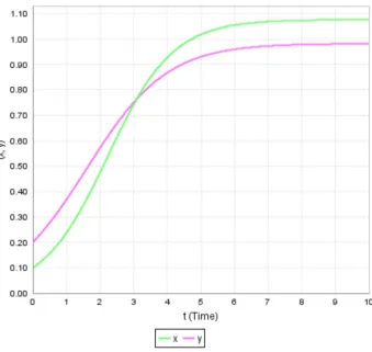
Figure 3. Dynamics of x and y populations starting with the higher initial value of x.
4. Results and Discussions
Figure 1 shows that the interior equilibrium point (1.0774, 0.98274) is a stable. This means that the solution trajectories tend to the equilibrium point without oscillation. This implies that at the given equilibrium point both populations can survive together.
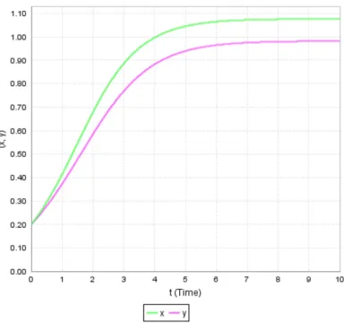
Figures 2-4 show the dynamics of both the populations with time. Moreover in these figures initial population sizes 0 = 0.2, 0.25, 0.1 and 0 = 0.2, 0.1, 0.25 respectively are considered and obtained the following results: If either the initial population sizes of both species are equal or if the initial population size of the first species is greater than the second species, then it can be observed that the growth rate of the first species dominates the growth rate of the second species. This fact is evident from Figures 2 and 3. If the initial population of the first species is less than the second species then continuous to dominate till the population sizes reach an equal value. After that starts dominating and this domination will continue forever.
Therefore, the unique positive equilibrium point D] ∗, ∗) = (1.0774, 0.98274) is globally asymptotically stable and both the species persist.
5. Conclusions
In this paper, a mutualism model in which the first population received benefit according to type II functional response and the second population received a benefit according to the type I functional response were considered. In addition to this functional response, the second population species was harvested with density dependent function or proportionally harvested has been presented. Based on the unique equilibrium point, the dynamical behavior of the population species considered and analyzed. In general from the numerical result, it can be observed that for any initial population the growth rate of the first population species dominate the second population species forever.
References
[1] L. H. Erbe, V. S. H. Rao and H. I. Freedman, “Three-species food chain models with mutual interference and time delays”, Math Biosci 80 (1986), 57–80.
[2] J. L. Bronstein, (1994). “Our current understands of mutualism”. Quarterly Review of Biology. 69 (1): 31–51. [3] M. Begon, J. L. Harper, and C. R. Townsend. 1996. “Ecology:
individuals, populations, and communities”, Third Edition. Blackwell Science Ltd., Cambridge, Massachusetts, USA.
[4] Morin. PJ, (2011). “Community ecology”, John Wiley and Sons, Hoboken, USA.
[5] Levins, R. 1966. “The strategy of model building in population biology”. American Scientist 54:421–431.
[6] MacArthur, R. H., and R. Levins. 1967. “The limiting similarity, convergence, and divergence of coexisting species”. American Naturalist 101:377–385.
[7] P. F. Verhulst, Recherches mathematiques sur la loi d'accroissement de la population [Mathematical researches into the law of population growth increase], Nouveaux Memoires de VAcademic Royale des Sciences et Belles-Lettres de Bruxelles, 18 (1845), 1—42.
[8] Freedman, H. I., “Deterministic Mathematical Models in Population Ecology”, Marcel Dekker, New York, USA 1980. [9] D. H. Wright, “A simple, stable model of mutualism
incorporating handling time”, The American Naturalist, 134 (1989), 664-667.
[10] J. Ollerton, 2006. “Biological Barter: Interactions of Specialization Compared across Different Mutualisms”. pp. 411–435 in: Waser, N. M. & Ollerton, J. (Eds) Plant-Pollinator Interactions: From Specialization to Generalization. University of Chicago Press.
[11] C. W. Clark, “Bio economic Modeling and Fisheries Management”, Wiley, New York, 1985.
[12] C. W. Clark, “Mathematical Bio economics: The Optimal Management of Renewable Resources”, Wiley, New York, 1990. [13] D. R. Jana, Agrawal, R. K. Upadhyay and G. P. Samanta,
“Ecological dynamics of age selective harvesting of fish population: Maximum sustainable yield and its control strategy”, Chaos, Solitons and Fractals 93 (2016), 111–122. [14] D. Jana, and G. P. Samanta, “Role of Multiple Delays in
ratio-dependent prey-predator system with prey harvesting under stochastic environment”, Neural, Parallel and scientific Computations 22 (2014), 205–222.
[15] T. R. Das, N. Mukherjee and K. S. Chaudhuri, “Harvesting of a prey–predator fishery in the presence of toxicity”, Appl Math Model 33 (2009), 2282–2292.
[16] M. Kot, “Elements of Mathematical Ecology”, Cambridge University Press, Cambridge, 2001.
[17] R. Ouncharoen, Pinjai S, Dumrongpokaphan T, and Lenbury Y (2012). “Global stability analysis of predator-prey model with harvesting and delay”. Thai Journal of Mathematics, 8(3): 589-605.