Published online February 20, 2014 (http://www.sciencepublishinggroup.com/j/ajep) doi: 10.11648/j.ajep.20140301.15
Calibrating the rainfall-runoff model GR4J and GR2M on
the Koulountou river basin, a tributary of the Gambia river
Vieux Boukhaly TRAORE
1, Soussou SAMBOU
1, Séni TAMBA
2, Sidy FALL
3,
Amadou Tahirou DIAW
4, Mohamed Talla CISSE
51Laboratoire d’Hydraulique et de Mécanique des Fluides (LHMF), Université Cheikh Anta Diop de Dakar (UCAD), Sénégal. BP 5005
Dakar-Fann
2Ecole Polytechnique de Thiès (EPT), BP 10 Thiès, Sénégal
3Office du Lac de Guiers, Société d’Aménagement et d’Exploitation des Terres du Delta du fleuve Sénégal et des Vallées du fleuve Sénégal
et de la Falémé (SAED)
4Laboratoire d’Enseignement et de Recherche en Géomatique (LERG); Campus Universitaire de l’Ecole Supérieure Polytechnique-Dakar ,
Sénégal. BP 5005 Dakar-Fann
5Université de Thiès. Thiès SENEGAL
Email address:
[email protected] (V. B. Traore)
To cite this article:
Vieux Boukhaly TRAORE, Soussou SAMBOU, Séni TAMBA, Sidy FALL, Amadou Tahirou DIAW, Mohamed Talla CISSE. Calibrating the Rainfall-Runoff Model GR4J and GR2M on the Koulountou River Basin, a Tributary of the Gambia River. American Journal of Environmental Protection. Vol. 3, No. 1, 2014, pp. 36-44. doi: 10.11648/j.ajep.20140301.15
Abstract:
Rainfall runoff modelling is the first step in water resources management. It is the only way to simulate the hydrological behavior of the basin for a good evaluation of the potentiality of this in term of water production. Many approaches are actually in use. In physically distributed models, deterministic relations issued from conservation laws of physics (mass conservation, moment momentum conservation) are solved to describe the hydrological processes generating flow and their interaction. A DEM that should be as complete as possible is associed. Complexity of the equations to be solved and the huge amount of required data, uncertainty in these data make these models of limited use. Conceptual rainfall-runoff models are often preferred by hydrologists. These models are based on equations relating in a realistic manner the different terms of the hydrological cycle. They are simpler than determistic models and more flexible, Conceptual models are generally global. According to the way hydrological cycle terms are taken into account, conceptual model can be classified as empirical or not. The aim of this paper is to evaluate the availability of water in the Koulountou river basin, a tributary of Gambia River. This river basin should reinforce the water resource in a neighboring Kayanga river basin. Two empirical models at daily and monthly scale, the GR4J and GR2M have been used to describe the hydrological behavior of this basin. These models have been realized by the CEMAGREF, a French research Office. They use as inputs daily or monthly rainfall and potential evapotranspiration and river basin area, and give as output daily or monthly runoff. The first step before applying a hydrological model is to calibrate it that is to estimate the best parameters that fit the outputs in a given period. The Nash criterion has been used as goodness-of-fit criterion. Model performs satisfactory when this criterion is greater than 0.70 according to available data. A period from 1971 to 1994 has been selected. This period have been divided into three parts: one for calibration (1971-1978), one for validation (1978-1986), and the last for application (1987-1994). The results we obtain shows that GR4J and GR2M performs well in the Koulountou river basin since the Nash criterion is greater than 0.8.Keywords:
Rainfall-Runoff Models, GR4J, GR2M, Validation, Calibration, Nash criterion, Koulountou River Subbasin, Gambia River basin1. Introduction
Assessment and effective management of water resources in a watershed requires a thorough understanding of
American Journal of Environmental Protection 2014; 3(1): 36-44 37
disciplines use models to describe systems in simpler terms and to predict systems response [2]. The choice must be made by identifying a parsimonious model structure which capture the dominant hydrological processes and provides good predictive power [3].In recent decades, many hydrological models have been developed [4] to represent a simple manner the natural systems [5].These models allow to estimate the part of rain that leaves the watershed knowing the rain it receives [6]. Rainfall-runoff models are important tools used in operational hydrology; they enable users to forecast or predict runoff of a catchment from the amount of precipitation received by this catchment [2].This
runoff in river catchment depends on how
topography-geomorphology, soils and vegetation, land use and land cover and climate changes interact [7]. From the spatial point of view, hydrological models are classified as lumped, semi-distributed, and distributed [8]. According to the relationships used to describe the physical processes, rainfall-runoff models are empirical, conceptual and physically based [9]. In lumped models, catchment is taken as a whole: spatial variability of vegetation, soil, and topography are ignored [9]. Runoff is estimated only at the catchment outlet [10]. Lumped models have a simple structure and empirical parameters. They require minimum data and are easy to use because of their fast setup and calibration [6]. Distributed models account for the heterogeneity and spatial variability of the catchment [1]. Such models give the closest representation of the real system; they incorporate as many components of actual physical processes as possible. Their calibration is highly time consuming because these models require huge data and model parameters identification [11, 12]. Though these parameters have a physical meaning, they are difficult to calculate; this may limit their strength and their adequacy for operational purposes [10, 13]. Semi-distributed models are a compromise between distributed process models and lumped models [10].They are less demanding on data than distributed models, present the advantage of simulating the values of different hydrologic variables at many points of the basin [14].Conceptual models use simplified mathematical relationships to represent the hydrological processes in the catchment. These models have a simple structure, and their data requirements are lower. They need fewer parameters, although these parameters have little physical sense. These models are of easy application, what make them important for flood forecasting, water resources planning, and water resources management ([9,14]. Conceptual models represent the component processes of the hydrological cycle by interconnected storage volumes [14]. Physically based models are based on governing equations such as conservation of mass and momentum equations in the description of hydrological processes. They require input of initial and boundary conditions since flow processes are described by differential equations [5]. Parameters and state variables of these models have a physical signification and
may either be directly measured in the field or reasonably assumed based on site characteristics. In these models, predictions are calculated where they are needed. These models are usually very complex; require an enormous data requirement and large computational demands, what is their main inconvenient [14]. Empiric models have no theoretical basis. They are mathematically simpler than the conceptual and physical models: they use statistical or similar technics to link observed inputs (rainfall) and output (discharges), their formulation needs little or no consideration of hydrologic cycle [15].
In this paper, we look for the feasibility of transferring water from Koulountou basin to the Kayanga basin. An understanding of the hydrologic behavior of these two basins is required. A first step is to select and run a rainfall-runoff model able to generate runoff at the outlet of each basin knowing rainfall and physical features. Distributed physically based are the best tool in such case, but as we pointed it earlier, they need to solve numerically the physical laws of conservation, are huge data demanding and time consuming and difficult to calibrate. Accounting for the available information, empiric global models are more suitable for us. These models are very little demanding in data, are very easy to calibrate. An example of such models is the “Génie Rural” models, developed by the French Research Center CEMAGREF. These models use as inputs the area of the basin, the potential evapotranspiration (E), and mean rainfall observations (P) over the whole basin. They give as outputs runoff at the outlet of the basin. These models run at monthly (GR2M) and daily (GR4J) time scale. We present the calibration and validation of the GR2M and GR4J in the Koulountou river basin. Results we obtain are satisfactory according to the Nash criterion.
2. Materials and Methods
2.1. Study Area
2.2. Description of the Models: GR4J and GR2M
The choice of a hydrological model for hydrologic applications in a given basin is a challenge. The available information is of great importance. In this s
information we have is the area of the basin and times series of rainfall and runoff. This oriented us towards lumped empiric hydrologic model that acts as input
Two of these are the GR4J and GR2M developed at the French CEMAGREF [16, 17].These models work at daily and monthly scale, are parsimonious in data and of easy calibration and validation what make them ve
among hydrologist [18, 19].We present the main features of
these models in the following.
2.2.1. Description of GR4J
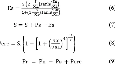
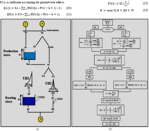
GR4J is divided into two stores: a production store and a routing store (Figure 2a). Computational
Figure 2b. Inputs of the model for a given day are rainfall P (mm) and potential evapotranspiration E (mm).
If P > E, then net rainfall Pn is given by
evaporation En by (2). A part Ps (3) of Pn is directed towards the production store, whose the maximum water content is the parameter X1 (mm) and actual content
Pn P E
En 0
Ps . . .
Figure 1. Koulountou River basin
: GR4J and GR2M
The choice of a hydrological model for hydrologic applications in a given basin is a challenge. The available information is of great importance. In this study, the only information we have is the area of the basin and times series of rainfall and runoff. This oriented us towards lumped empiric hydrologic model that acts as input-outputs models. Two of these are the GR4J and GR2M developed at the ].These models work at daily and monthly scale, are parsimonious in data and of easy calibration and validation what make them very popular We present the main features of
GR4J is divided into two stores: a production store and a Computational details are given in Inputs of the model for a given day are rainfall P
E (mm).
given by (1) and net of Pn is directed towards the production store, whose the maximum water content is
ter X1 (mm) and actual content is S (mm).
(1)
(2)
(3)
The remaining part Pn-Ps is
If P< E, the net evaporation is equal to (4) and net rainfall to (5).
En Pn
A part Es (6) of En is extracted whose actual content is updated by is taken from this updated content
and added to the direct runoff part of rainfall to giv which is the total water available for the routing
Es . ..
S S ! Ps
Perc S. %1 '1
Pr Pn
Pr is then divided into two parts, one part (10%) for direct runoff Q1 (10) through unit hydrograph HU2 with base time equal to 2X4; the other part, (90%) for de
(11), which reaches the routing store through unit hydrograph HU1 with base tim
of the routing store is X3. Its actual conte using Q9 and the value of the function F(X2) (12
Ps is reserved to calculate runoff. P< E, the net evaporation is equal to (4) and net rainfall
E P (4)
Pn 0 (5) acted from the production store is updated by (7). Percolation Perc (8) updated content of the production store and added to the direct runoff part of rainfall to give Pr (9)
otal water available for the routing.
(
. ( (6)
Es (7)
' ! * ) )+ ,
-. (8)
American Journal of Environmental Protection 2014; 3(1): 36-44 39
X2 is a coefficient accounting for groundwater effects.
Q1 i 0.1 1 ∑ HU2 k 1 Pr i k ! 1 17
89: (10)
Q9 i 0.9 1 ∑ HU1 k 1 Pr i k ! 1 <
89: (11)
F X2 X2 ?@ A (12)
R max 0, R ! Q9 ! F (13)
Figure 2. GR4J Model Structure (a); Computation organization (b)
Then this updated content of routing store is used to calculate the final delayed output Qr (14) of the routing store. Q1 and F(X2) are combinated to calculate the direct runoff Qd (15). Total runoff for the given day at the outlet of the basin, is then estimated by summing Qr and Qd (16). Since the works of Perrin [16, 19, 20], many authors have brought contributions to that model [21, 22, 23].
Qr R. %1 '1 ! @? )+
,
-. (14)
Qd max 0, Q1 ! F (15)
Q Q ! Qd (16) 2.2.2. Description of GR2M
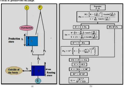
GR2M is an empirical lumped monthly hydrologic model working with two stores (Figure 3a): a production store whose capacity is the parameter X1 and actual contents is S;
and a routing store whose capacity is set to 60 mm and actual contents is R [17].Inputs of the model are monthly rainfall (P) and potential evapotranspiration (E) for a given month and output is monthly runoff at the outlet of the basin Q. A part Ps (17) of rainfall P is directed to production store, whose content becomes S’ given by (18). The excess part P1 (19) is directed to the routing store.
Ps . . . (17)
P P P (18)
Percolation given by (22).
Es . II.. (( (20)
SJJ SJ E (21)
P SJJ. %1 '1 ! II @+
, K
. (22)
P2 is added to the routing store. Total water P3 input of the
routing store is then given by (23), and its content pass to R’ given by (24).
At this step, a fraction X2R’ of R’ is reserved for the
routing store, and the difference F (25) is taken away from the basin as groundwater exchange.
P@ P ! P (23)
RJ R ! P3 (24)
F= (X2-1) R’ (25)
The level in the routing store becomes R’’ (26). Then the output runoff Q is estimated by (27): [24, 25]. Computation organization is presented in ( figure3b).
R’’ RJ! F (26)
Q ??IIIIMN (27)
Figure 3. GR2M model Structure (a)
;
Computation organization (b)2.4. Models Calibration and Validation
Parameters of empirical models have a meaning that is not connected a priori to measurable quantities of the watershed [7]. So, their calibration is required. Calibration is the process of choosing best sets of model parameters, by adjusting manually or automatically their numerical values to better mimic the response observed at the outlet [26]. The successful application of a hydrologic watershed model depends on how well the model is calibrated [5]. The calibrated models parameters should necessarily be validated. Validating a model is to the check the
American Journal of Environmental Protection 2014; 3(1): 36-44 41
NashQ 100 Q1 ∑ RSTUV RSWXY
∑ R[[[[[[[ RZTUV SWXY \
(28)
Nash]Q 100 ^ _ _ `
1 ∑abRS
TUV bR S WXY c
∑dbR[[[[[[[[[[ZTUV bR S WXYe
f g g h
(29)
NashlogQ 100 Q1 ∑ :lmRSTUV :lmRSWXY
∑ :lmR[[[[[[[[[[[[ :lmRZTUV S
WXY \ (30)
Qnlop daily flow observed on day i; Qq :n : daily rate
calculated on day i; [[[[[[Qrlop : average rate observed during the simulation period. A value of Nash equal to 0 or less than 0 indicates a very bad correlation: it shows that observed mean is better than simulated mean; a value of Nash equal to 1 corresponds to a perfect model, which reproduces reality: it shows complete adaptation is between observed mean and simulated mean. In practice the value of 0.70 is taken as the threshold: below this value, simulation is bad and beyond, it is good [30].
3. Application
3.1. Data
Data used in this application are daily rainfall and daily flow at the stream gauge station of Missirah Gounass, outlet of the catchment, and potential evapotranspiration at the station of Kédougou on the Gambia River. These data are issued from the database of OMVG (Organization for the development of the Gambia River) shared by the countries of Guinea, Gambia and Senegal. The period extending from 1971 to 1994 has been selected. This period has been divided into three parts for calibration (1971-1978), validation (1978-1986), and application (1987-1994).
3.2. Calibration, Validation and Application of the GR2M and GR4J Models
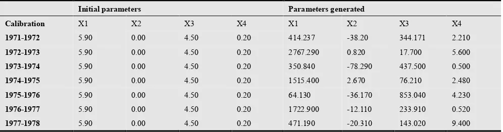
We first generate a set of parameters of each of these models for each year of the calibration periods (1971-1978) using the Excel version. Each of these set of parameters is applied to the whole period of calibration using the FORTRAN executable version of these models, and the different Nash criteria (1), (2), (3) are calculated. Set of parameters corresponding to the best Nash values are then considered as models parameters. These parameters are then applied to the validation period (1979-1987) to verify if they are well suited, and then on the application period (1988-1994) to confirm the results.
Table 1. Parameters generated in the period1971-1978 withGR4J
Initial parameters Parameters generated
Calibration X1 X2 X3 X4 X1 X2 X3 X4
1971-1972 5.90 0.00 4.50 0.20 414.237 -38.20 344.171 2.210 1972-1973 5.90 0.00 4.50 0.20 2767.290 0.820 17.700 5.600 1973-1974 5.90 0.00 4.50 0.20 350.840 -78.290 437.500 0.500 1974-1975 5.90 0.00 4.50 0.20 1515.400 2.670 76.210 2.480 1975-1976 5.90 0.00 4.50 0.20 64.130 -36.170 853.040 4.230 1976-1977 5.90 0.00 4.50 0.20 1722.900 -12.110 233.910 0.520 1977-1978 5.90 0.00 4.50 0.20 471.190 -20.310 143.020 9.400
3.3. Results and Discussion
3.3.1. Calibration and Validation of the GR4J and GR2M In Tables 1 and 2 we have presented set of parameters on the calibration period (1971-1978) generated from the Excel version. The data of first year (for example 1971) are used to generate the set parameters corresponding to the second year (for example 1972). In tables 3 and 4, we present the criteria
obtained when each set of parameters is applied to the whole validation period. Examination of the Nash criterion outlines the best set of parameters for each of the model. These parameters will be considered a priori for both models as optimal parameters for basin Koulountou Missirah Gounass which is the most downstream station.
Table 2. Parameters generated in the period1971-1978 withGR2M
Initial parameters Parameters generated
Calibration X1 X2 X1 X2
1971-1972 6 1 168.30 0.79
1972-1973 6 1 3.48 0.77
1973-1974 6 1 5.33 0.71
1974-1975 6 1 2.37 0.86
1975-1976 6 1 2.09 0.85
1976-1977 6 1 22.09 0.76
Table 3. Research of best set parameters with GR4J
Generated parameters Nash criteria
Validation X1 X2 X3 X4 NashQ Nash√Q NashlogQ
1978-1986
414.237 -38.20 344.171 2.210 0.0248 0.5285 0.6752
2767.29 0.820 17.700 5.600 -1.5313 -0.8466 -0.8193
350.840 -78.290 437.500 0.500 0.8355 0.9072 0.8993
1515.400 2.670 76.210 2.480 -4.0200 -1.3222 -0.8502
64.130 -36.170 853.040 4.230 -1.9776 -0.3585 -0.1485
1722.900 -12.110 233.910 0.520 0.3038 0.4359 0.3531
471.190 -20.310 143.020 9.400 -0.0971 0.5035 0.7633
Table 4. Research of best set parameters withGR2M
Generated parameters Nash criteria
Validation X1 X2 NashQ Nash√Q NashlogQ
1978-1986
168.30 0.79 0.190 0.382 0.209
3.48 0.77 0.586 0.549 0.345
5.33 0.71 0.866 0.864 0.760
2.37 0.86 -2.447 -0.883 -0.672
2.09 0.85 -2.470 -0.861 -0.629
22.09 0.76 0.656 0.794 0.735
173.86 0.73 0.056 0.356 0.442
3.3.2. Application Period
The best set parameters obtained for each model on the validation period are applied to the application period for verification. As 1991 is missing, this period was divided into two sub-periods: 1987-1990 and 1992-1994. We show the whole results for the two models in Tables 5 and 6. According to these tables, Nash criteria are all greater than 0.70 so that the set of parameters can be considered as
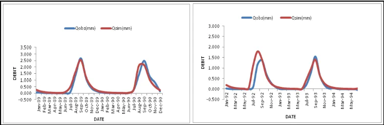
representative for the Koulountou basin and significant for each of the models. They can be used to simulate flow in the Koulountou river basin at the stream gauge of Missirah Gounass at daily (for GR4J) and monthly (for GR2M). Simulated and observed flows for the application period are compared in Figure 4 and 5. There is a generally good fitness.
Table 5. Optimal parameters for the period1987-1994 with GR4J
Optimal parameters Nash criteria Application
Phase1:(1987-1990) X1 X2 X3 X4 NashQ Nash√Q NashlogQ
350.840 -78.290 437.500 0.500 0.7976 0.8988 0.8706
Phase2 :(1987-1990)
350.840 -78.290 437.500 0.500 0.8473 0.8803 0.8520
Table 6. Optimal parameters for the period1987-1994 with GR2M
Optimal parameters Nash criteria Application
Phase1:(1987-1990) X1 X2 NashQ Nash√Q NashlogQ
5.33 0.71 0.929 0.924 0.849
Phase2:(1992-1994)
5.33 0.71 0.806 0.887 0.849
American Journal of Environmental Protection 2014; 3(1): 36-44 43
Figure 5. Validation of GR2M on phase 1(a) and phase 2(b)
4. Conclusion
Water resources management requires well calibrated and validated rainfall runoff models. Physical based models are well suited, but they have they present the inconvenient to be very difficult to implement: they are highly data demanding and very difficult to calibrate. Empirical global models are of easy calibration and application. In this paper, we aim at evaluating water resource of the Koulountou river Basin, a left side tributary of the Gambia River to reinforce the water resource in a neighboring river basin, the Kayanga river basin. According to the available data, we have used lumped empirical daily and monthly models, the GR4J and GR2M models developed by the French CEMAGREF. Calibration have been made by first generated in the calibration period, then applied in each year of this calibration period. Nash criteria have then been used to choose the best set of parameters for each model. Application of these best sets in the validation period gave a good adequation between calculated and observed according to the Nash criteria for the two models. To confirm these results, we have used the same parameters to simulate flows in an application period different of the calibration and validation periods. Once again, Nash criteria and plots show a good agreement between the values of simulated and observed flows. The work made in this paper has allowed us to determine the best set of parameters for the application of GR4J and GR2M models in the Koulountou river basin. These parameters can be used to restore missing flows from rainfall, and particularly to assess the water resources trends in the future horizons
.
Acknowledgements
We thank particularly Mr Lamine KONATE from OMVG who helped us to use the data base.
References
[1] Koffi, F.K. and Monique BERNIER, Droh L. GONÉ, Mahaman B. SALEY, René LEFÈBVRE, Nagnin SORO et Aimé KOUDOU, (2007) «Integrating geo space in a distributed hydrological model for the simulation of water flow in the humid tropics of Ivory Coast (West Africa) »."
Journal Remote Sensing, 2007, vol. 7, No. 1-2-3-4, pp. 217-23
[2] Donelly-Makowecki, L. M. and Moore, R. D., (1999) «Hierarchical testing of three rainfall-runoff models in small forested catchments ». Journal of Hydrology, 219(3/4), 136-152.
[3] Hilary McMillan, Martyn Clark, Ross Woods, Maurice Duncan, MS Srinivasan, Andrew Western & Dave Goodrich, (2010) « Improving perceptual and conceptual hydrological models using data from small basins». IAHS Publ. 336, pp. 264-269
[4] Singh, V.P. and Woolhiser, D.A.,(2002) « Mathematical modeling of watershed hydrology ». Journal of Hydrologic Engineering, vol. 7, n° 4, p. 270-292
[5] Dilip Kumar, (2011) « Distributed rainfall Runoff modeling». International journal of earth sciences and engineering, pp.270-275
[6] K.Narasayya,U.C.Roman, B.L.Meena, S.Sreekanth, S.Naveed Ali, (2013) «Prediction of storm-runoff using physically based hydrological model for burhanpur watershed, India » International journal of remote sensing and geosciences (IJRSG), vol.2, pp.76-85
[7] Zhiyu Liu and Ezio Todini, (2002) « Towards a comprehensive physically-based rainfall model ».Hydrology and Earth system sciences,6(5), pp . 859-881
[8] Yuyu Zhou and Y.Q.Wang,(2008) « a distributed and object-oriented rainfall-runoff simulation model with hich spatial resolution impervious surface » .annual conference Portland, Oregon, pp.1-12.
[9] Md. Sharif Imam Ibne Amir, Mohammad Masud Kamal Khan, Mohammad Golam Rasul, Raj H. Sharma, and Fatema Akram,(2013) « Automatic multi-objective calibration of rainfall runoff model for the Fitzroy basin, queensland, Australia ». International journal of environmental science and development, vol 4, pp .311-315
[10] Vahid Nourani, Arash Roughani and Mekonnen Gebremichael, (2011) « TOPMODEL Capability for rainfall-runoff modeling of the ammameh watershed at different time scales using different terrain algorithms». Journal of urban environment engineering, vol.5.n.1, PP.1-14
[12] P.C. Shakti, N.K. Shrestha and P. Gurung, (2010) « Step wise multi-criteria performance evaluation of rainfall-runoff models using WETSPRO » Journal of hydrology and meteorology,vol.7 ,pp.18-29
[13] APIP, Takahiro SAYAMA, Yasuto TACHIKAWA and Kaoru TAKARA,(2008) « Lumping of physically-based distributed model for sediment runoff prediction in a catchment scale» annual journal of hydraulic engineering, JSCE, vol.52, PP.43-47
[14] XU,Z.X.,Takeuchi,K.,and Ishidaira,H.,(2002) « A conceptually based-distributed rainfall-runoff model applied in arid regions » .International conference on urban hydrology for the 21st century pp.45-60
[15] Kokkonen, T. S., and A. J. Jakeman,(2001) « A comparison of metric and conceptual approaches in rainfall-runoff modeling and its implications ».Water Resources Research 37(9), pp. 2345– 2352
[16] Perrin, C., Michel, C., Andréassian, V., (2003) « Improvement of a parsimonious model for streamflow simulation». Journal of Hydrology, 279(1-4), pp. 275-289.
[17] Makhlouf, Z.and Michel, C., (1994) « A two-parameter monthly water balance model for French watersheds ». Journal of Hydrology 162, 299-318.
[18] Huard, D. and A. Mailhot ,(2008) « Calibration of hydrological model GR2M using Bayesian uncertainty analysis ». Water Resour.Vol 44, W02424, pp.1-19.
[19] Perrin, C. and Littlewood, I.G. (2000) « A comparative assessment of two rainfall-runoff modelling approaches: GR4J and IHACRES». Proceedings of the Liblice Conference (22-24 September 1998), V. Elias and I.G. Littlewood (Eds.), IHP-V, Technical Documents in Hydrology n° 37, UNESCO, Paris, pp. 191-201.
[20] Perrin, C., Michel, C. et Andréassian, V., (2001) «Does a large number of parameters enhance model performance? Comparative assessment of common catchment model structures on 429 catchments ». Journal of Hydrology, 242(3-4),pp .275-301.
[21] Le Moine, N., V. Andréassian, C. Michel & C. Perrin, (2005) «How to Account For Groundwater Exchanges In Rainfall-Runoff Models In Zerger, A. and Argent, R.M.(eds)
MODSIM » International Congress on Modelling and Simulation. Modelling and Simulation Society of Australia and New Zealand, pp. 2932-2938
[22] Oudin,L.F. Hervieu,C.Michel, C.Perrin,V.Andreassian, F.Anctil and C. Loumagne (2005) « Which potential evapotranspiration input for a lumped rainfallrunoff model?: Part 2-Towards a simple and efficient potential evapotranspiration model for rainfall-runoff modeling ». Journal of Hydrology 303(1-4),pp. 290-306
[23] Dhemi Harlan, Muljana Wangsadipura., and Cecep Muhtaj Munajat,( 2010) « Rainfall-runoff modeling of citarum hulu river basin by using gr4j». Proceedings of the World Congress on Engineering 2010 Vol II,pp. 1-5.
[24] Mouelhi,S. , Michel, C., Perrin, C. et Andréassian V,(2006) « Stepwise development of a two parameter monthly water balance model ».J. Hydrol. 318(1-4), 200-214.
[25] Maryam Zolfaghari, Mohamad Mahdavi, Ali Rezaei, Ali Salajegheh,(2013) « Evaluating GR2M Model in Some Small Watersheds of Iran (Case Study Gilan and Mazandaran Provinces) ». Journal of Basic and Applied Scientific Research; 3(2), pp. 463-472.
[26] Madsen, H., G. Wilson, and and H. C.Ammentorp, (2002) « Comparison of different automated strategies for calibration of rainfall-runoff models». Journal of Hydrology 261(1-4) pp .48-59.
[27] Nash, J.E. and Barsi, B.I., (1983) «A hybrid model for flow forecasting on large catchments» .J. Hydrol., 65, pp .125-137.
[28] Krause, P., Boyle, D. P., Base, F., 2005, Comparison of different efficiency criteria for hydrological model assessment, Advances in Geosciences, Vol: 5, pp .89–97
[29] Loumagne, C., Michel, C., Palagos, B., Baudez, J.C. and Bartoli, F. (1999) « From a global to a semi-distributed approach in rainfall-runoff modelling ». La Houille Blanche, 6, pp .81-88