http://www.sciencepublishinggroup.com/j/ijdsa doi: 10.11648/j.ijdsa.20190501.11
ISSN: 2575-1883 (Print); ISSN: 2575-1891 (Online)
An Estimation of Unknown Variance of a Normal
Distribution: Application to Borno State Rainfall Data
Adegoke Taiwo Mobolaji
1, Nicholas Pindar Dibal
2, Yahaya Abdullahi Musa
21
Department of Statistics, University of Ilorin, Ilorin, Nigeria
2Department of Mathematical Sciences, University of Maiduguri, Maiduguri, Nigeria
Email address:
To cite this article:
Adegoke Taiwo Mobolaji, Nicholas Pindar Dibal, Yahaya Abdullahi Musa. An Estimation of Unknown Variance of a Normal Distribution: Application to Borno State Rainfall Data. International Journal of Data Science and Analysis. Vol. 5, No. 1, 2019, pp. 1-5.
doi: 10.11648/j.ijdsa.20190501.11
Received: December 26, 2018; Accepted: February 15, 2019; Published: March 28, 2019
Abstract:
The Bayesian estimation of unknown variance of a normal distribution is examined under different priors using Gibbs sampling approach with an assumption that mean is known. The posterior distributions for the unknown variance of the Normal distribution were derived using the following priors: Inverse Gamma distribution, Inverse Chi-square distribution and Levy distribution of the unknown variance of a normal distribution and Gumbel Type II. R functions are developed to study the various statistical simulation samples generated from Winbugs.Keywords:
Normal Distribution, Prior Distribution, Posterior Distribution, Bayesian Estimation,Inverse Gamma Distribution, Inverse Chi-Square Distribution, Levy Distribution, Gumbel Type II Distribution
1. Introduction
In statistical inference, there are two broad categories of interpretations of probability: Bayesian inference and frequentist inference. These views often differ with each other on the fundamental nature of probability. Frequentist inference loosely defines probability as the limit of an event’s relative frequency in a large number of trials, and only in the context of experiments that are random and well-defined.
Bayesian inference, on the other hand, is able to assign probabilities to any statement, even when a random process is not involved. In Bayesian inference, probability is a way to represent an individual’s degree of belief in a statement, or given evidence.
In frequentist approach, a general method for calculating statistics that estimate specific parameters is called Maximum Likelihood (ML). This method is considered to be more robust (with some exceptions) and yields estimators with good statistical properties, it is perhaps the most versatile method for fitting statistical models to data, it finds the value of one or more parameters for a given statistic which makes the known likelihood distribution a maximum [14].
In typical applications, the goal is to use a parametric statistical model to describe a set of data or a process that generated a set of data. The appeal of ML stems from the fact that it can be applied to a wide range of statistical models and kinds of data (e.g., continuous, discrete, categorical, censored, truncated, etc.), where other popular method, like least squares, do not, in general, provide a satisfactory method of estimation. Indeed, when assuming an underlying normal (also known as Gaussian) distribution, the least squares estimates of regression coefficients are equivalent to ML estimates. The ML method is, however, much more general because it allows one to use other distributions as well as more general assumptions about the model and the form of the data. This study focus on the estimation of variance of a Normal distribution under different prior distributions.
2. Materials and Methods
2.1. Data Description
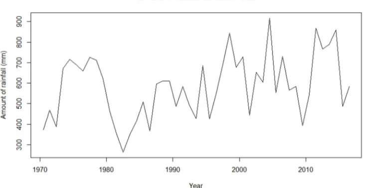
for Borno State. Appendix Figure 1 and Figure 2 show the time plot and qqplot for the amount of rainfall in Borno state.
Figure 1. Time plot graph for the amount of rainfall in Borno State.
Figure 2. QQplot for rainfall data of Borno state.
2.2. Methodology
The problem of estimation is to devise means of using sample observations to construct good estimates of one or more of the parameters. It is expected that the information in the sample concerning those parameters will make an estimate based on the sample generally better than a sheer guess. How well the parameter is approximated can depend on the method, the type of data and other factors. The method of maximum likelihood corresponds to many well-known estimation methods in statistics (such as; maximum likelihood, moments, least squares, Bayesian estimation etc) and finding particular parametric values that make the observed results the most probable (given the model).
Cox and Reid [2] used Composite Likelihood methods for approximating the likelihood function and also [1, 10] applied Approximate Bayesian Computational (ABC) methods for approximating the posterior distribution for
obtaining estimates of parameter. It is well-known that ABC produces a simple approximation of the posterior distribution [1] in which there exists a deterministic approximation error in addition to Monte Carlo variability. The quality of the approximation to the posterior and theoretical properties of the estimators obtained with ABC have been studied [3, 5, 7, 15]. The use of ABC posterior samples for conducting model comparison was studied [4, 12]. Using this sample approximation to characterize the mode of the posterior would in principle allow (approximate) maximum a posteriori (MAP) estimation.
2.3. Bayes Theorem
one has a probability function called prior distribution. The estimate of the unknown parameter is obtained by deriving a posterior distribution on the basis of the prior distributions and the likelihood function. The Bayesian methods allow the integration of statistical analysis through the prior distribution with the most current information based on the observations into a posterior distribution. In other words, the prior to experimentation; the posterior distribution, an updated belief about the parameters after sample data is obtained. The posterior distribution is obtained: Posterior ∝ likelihood × prior
σ | ∝ |σ × σ
2.4. Normal Distribution
The normal distribution is one of the most important probability distribution in statistics because it fits many natural phenomena.
Consider the probability distribution function of a random variable . , . ⋯ ⋯ , drawn from a normal distribution with mean and variance σ
; , σ = (1)
The likelihood function of (1) can be expressed as
, σ | = ! 1
√2%σ
&'
= ( )
*
∑*/0 ,-.
(2)
The aim of this study is to obtain an estimate for variance of a normal distribution using different prior distributions and to determine the efficient prior distribution by comparing the posterior variances.
2.4.1. Posterior Distribution of Unknown Parameter 12 Using Inverse Gamma Prior Distribution
[6, 9, 11, 13, 16] assumed an inverse gamma distribution for the parameter of interest σ of 3 normaldistribution with hyper parameters 3 345 6. The probability distribution function for the prior distribution can be expressed as
σ |3, 6 = 9 :78 σ :; < (3)
where a > 0, b > 0, σ > 0
To obtain the posterior distribution of σ | , we combined
equations (3) and (2).
σ | ∝ σ ?*;:; @ A7;∑ ,-. B
(4)
which results to a kernel density of an inverse gamma
distribution with parameters ? + 3,7;∑ @
2.4.2. Posterior Distribution of Unknown Parameter 12 Using Inverse Chi-Squares Prior Distribution
Obisesan [8] assumed an inverse chi-squares distribution for parameter σ with hyper parameterD and 5 which the distribution function can be expressed as
σ |D, 5 = 9?E@
F
GEHE σ
:; EF ; HIJ,GIJ (5)
To obtain the posterior distribution of σ | , we combined equations (5) and (2).
σ | ∝ σ ?*KE; @ AHG;∑ ,-. B
(6)
which results to a kernel density of an inverse gamma
distribution with parameters ? ;H, D5 +∑ @
2.4.3. Posterior Distribution of Unknown Parameter 12 Using Levy Prior Distribution
We assumed a Levy prior distribution with parameter e for the unknown parameter σ . The probability distribution function for the Levy prior distribution can be expressed as
σ | = LM σ N O ; > 0, σ > 0 (7)
To obtain the posterior distribution of σ | , we combined equations (7) and (2).
σ | ∝ σ ?*KN@ AOK∑ ,-. B (8) which results to a kernel density of an inverse gamma
distribution with parameters ? ; ,M;∑ @.
2.4.4. Posterior Distribution of Unknown Parameter 12 Using Gumbel Type II Prior Distribution
We assumed Gumbel Type II prior probability distribution with parameters f and g for unknown parameterσ , which has the following probability distribution functions
σ | , P = P σ Q;
R
S TU; > 0, P > 0, σ > 0 (9)
In order to make (13) a conjugate prior we take f = 1, then the prior distribution becomes
σ |P = P σ R ; P > 0, σ > 0 (10) To obtain the posterior distribution of σ | , we combined equations (10) and (2).
σ | ∝ σ ?*; @ AV;∑ ,-. B (11) which results to a kernel density of an inverse gamma
3. Results and Discussion
Table 1. Posterior Distribution of Variance using Inverse Gamma prior distribution.
Mean sd 2.5pc Median 97.5pc
a=b=05 26430 5124 18230 25820 38120
a=b=10 22320 3970 15920 21850 31380
a=b=15 19420 3247 14080 19090 26690
a=b=20 17070 2646 12660 16800 23050
Table 2. Posterior Distribution of Variance using Inverse Chi-square prior distribution.
Mean sd 2.5pc Median 97.5pc
a=b=05 29100 5975 19640 28320 42830
a=b=10 26430 5124 18230 25820 38120
a=b=15 24240 4493 16900 23770 34450
a=b=20 22320 3970 15920 21850 31380
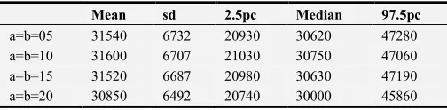
Table 3. Posterior Distribution of Variance using Levy prior distribution.
Mean sd 2.5pc Median 97.5pc
a=b=05 31540 6732 20930 30620 47280
a=b=10 31600 6707 21030 30750 47060
a=b=15 31520 6687 20980 30630 47190
a=b=20 30850 6492 20740 30000 45860
Table 4. Posterior Distribution of Variance using Gumbel Type II prior distribution.
Mean sd 2.5pc Median 97.5pc
a=b=05 30850 6492 20740 30000 45860
a=b=10 29640 6083 20090 28860 43830
a=b=15 29630 6197 19900 28800 43880
a=b=20 28500 5775 19350 27800 41740
Tables 1-4, shows the posterior variances under the various informative prior distributions with assumed values of hyper parameters. The length of the burn-in period is 1,000 and the number of iterations of the Gibbs sampler after the burn-in period is chosen as 9,000. From the results displayed in Tables 1-4, we observed that the posterior variances under the inverse gamma distribution less compare with other informative distribution which proves that the inverse gamma distribution is efficient as compared to other priors.
4. Conclusion
In this research work, we compare different conjugate prior distribution for the unknown parameter variance of a normal distribution. Four conjugate prior distributions were considered namely: inverse gamma distribution, inverse chi-squares distribution, Gumbel Type II prior distribution and Levy prior distribution. Posterior distributions for variances were derived under the four conjugate prior distribution. Comparison were made using the estimated variances obtained under the four conjugate prior distribution and we conclude that inverse gamma distribution performs better than the other three prior distributions. So therefore, we recommend that inverse gamma distribution should be used
when estimating the unknown variance of normal distribution.
Acknowledgements
The authors are grateful to anonymous reviewers for their valuable comments on the original draft of this manuscript.
References
[1] Beaumont, M. A., Zhang, W. and Balding, D. J. (2002). Approximate Bayesian computation in population genetics. Genetics, 162, 2025-2035.
[2] Cox, D. R. and Reid, N. (2004). A note on pseudo likelihood constructed from marginaldensities. Biometrika, 91, 729-737. [3] Dean, T. A., Singh, S. S., Jasra A. and Peters G. W. (2011).
Parameter estimation for hidden Markov models with intractable likelihoods. Arxiv preprint arXiv: 1103.5399v1. [4] Didelot, X., Everitt, R. G., Johansen, A. M. and Lawson, D. J.
(2011). Likelihood-free estimation of model evidence. Bayesian Analysis, 6, 49-76.
[5] Fearnhead, P. and Prangle, D. (2012). Constructing Summary Statistics for Approximate Bayesian Computation: Semi-automatic ABC (with discussion). Journal of the Royal Statistical Society.
[6] Kelvin P. Murphy (2017). Conjugate Bayesian analysis of the Gaussian distribution. Handbook on Bayesian Statistics, 1-29. [7] Marin, J., Pudlo, P., Robert, C. P. and Ryder, R. (2011).
Approximate Bayesian Computational methods. Statistics and Computing.
[8] Obisesan, K. (2015). Change-point detection in time series with hydrological applications. Master’s thesis, University College London.
[9] Perreault, L., Bernier, J., Bobee B., Parent, E. (2000), Bayesian change-point analysis in hydro meteorological time series. Part 1. The normal model revisited. Journal of Hydrology 235, 221–241.
[10] Pritchard, J. K., Seielstad, M. T., Perez-Lezaun, A., and Feldman, M. T. (1999). Population Growth of Human Y Chromosomes: A Study of Y. Chromosome Microsatellites. Molecular Biology and Evolution 16: 1791 1798.
[11] Rebecca C. Steorts, (2016). Baby Bayes using R.
[12] Robert, C. P., Cornuet, J., Marin, J. and Pillai, N. S. (2011). Lack of confidence in ABC model choice. Proceedings of the National Academy of Sciences of the United States of America 108: 15112–15117.
[13] Tendor Mihai Moldovan, (2010). The Conjugate Prior for the Normal Distribution, Technical report, 1-6.
[14] Weisstein, E. W. (2012). Maximum Likelihood. From MathWorld—A Wolfram Web Resource. http://mathwor ld.wolfram.com/MaximumLikelihood.html.