Published online March 10, 2013 (http://www.sciencepublishinggroup.com/j/ajee) doi: 10.11648/j.ajee.20130101.11
A proposed algorithms for tidal in-stream speed model
Hamed H. H. Aly, M. E. El-Hawary
Department of Electrical and Computer Engineering, Dalhousie University, Halifax, Nova Scotia, Canada, B3H 4R2
Email address:
[email protected] (H. H. H. Aly,), [email protected] (M. E. El-Hawary)
To cite this article:
Hamed H. H. Aly, M. E. El-Hawary. A Proposed Algorithms for Tidal in-Stream Speed Model. American Journal of Energy Engineering. Vol. 1, No. 1, 2013, pp. 1-10. doi: 10.11648/j.ajee.20130101.11
Abstract:
In this paper we propose four models for tidal current speed and direction magnitude forecasting model. The first model is a Fourier series model based on the least squares method (FLSM), the second model is an artificial neural network (ANN), the third model is a hybrid of FLSM and ANN and the fourth model is a hybrid of ANN and FLSM for monthly forecasting of tidal current speed. These proposed models are ranked in order depending on their performance. These models are validated by using another set of data (tidal current direction). The proposed hybrid model of FLSM and ANN is highly accurate and outperforms. This study was done using data collected from the Bay of Fundy in 2008.Keywords:
Power System Modeling, Tidal Currents, Forecasting, ANN, Fourier Series Based On Least Squares1. Introduction
Tidal current energy can be converted into electrical power. It is so hard to store the electrical energy for later use and a control system is required to be connected direct-ly to the consumer. It is very important to have advance knowledge of the tidal current energy to manage the pro-duction of the electrical power so that it may ensure that this power will be controlled in an efficient way to allow scheduling different electrical energy resources to minimize interruptions. Prior knowledge of future generated electrical energy or the tidal current energy is known as forecasting. Tidal flow causes somewhat predictable energy output pat-terns. Forecasting marine currents using data gathered for short periods of time is predictable to within 98% accuracy). On the other hand forecasting wind speed requires data gathered over a longer period. The marine resource is easier to integrate in the electrical grid. Forecasting is the first step in dealing with the future generation of the tidal cur-rent power systems. The accuracy of the models used for tidal current forecasting is critical as a tidal in-stream fore-cast with sufficient accuracy can provide a stable and con-trolled electric power dynamic performance that allows better dispatching of grid resources and this evens out the use of battery storage and will affect the overall cost of electricity. In addition, tidal current prediction is useful in making operations- and planning related decisions such as towing of activities vessels, fisheries and recreational ac-tivities and monitoring of oil slick movements [1, 2].
2. Previous Research for Tidal Currents
Forecasting
Sir G. H. Darwin [3] is credited with the idea that tidal oscillation of the ocean may be represented as the sum of a number of simple harmonic waves. Subsequently, Doodson [4-5] proposed using least squares estimation to determine the parameters of the harmonic series which has been wide-ly used for tidal forecasting [6].
other two field data of diurnal and mixed types were used to test the performance of a PBN model.
Vijay and Govil [15] used radial basis function ANN networks (RBF) for tidal data prediction of high and low tides of any day of the year depending on the training data of only one month. They concluded that a Fourier series or a polynomial series alone do not give accurate results. They also reported that using Wavelets yielded approximately the same results as ANN but implementing the Wavelet ap-proach required longer execution time. Chen, Wang and Chu [16] proposed a hybrid of wavelet and ANN models for tidal current prediction. The signal in the multi-resolution analysis (MRA) used in wavelet analysis consists of high and low frequency components. Chen et al. elimi-nated the high frequency components and used the inverse wavelets to rebuild new signals. The input/output data that were used for the training of the ANN depended on the cal-culation of the tidal constituent time-lags. Adamowski [17] proposed a hybrid of ANN and wavelet and cross wavelet constituent components for short term river flood forecast-ing that gave accurate results compared to wavelet and cross wavelet constituent components alone.
In [18] genetic algorithms (GA), were used to carry out the prediction task. A preliminary empirical orthogonal function (EOF) analysis was used to compress the spatial variability into a few eigen-modes, so that GA could be applied to the time series of the dominant principal compo-nents (PC). Burrage et al. proposed an optimal multi linear regression model for the tidal current forecasting [19].
Harmonic tidal current constituent analysis or numerical hydrodynamic models are traditional models used for tidal current prediction. These models have their own limitations and nonlinear data adaptive approaches are gaining in-creased acceptance. Numerical hydrodynamic models re-quire large computing resources and huge input information.
In this paper such an approach, known as a Hybrid model, has been employed for the tidal prediction. The novelty of the method is the use of the ANN or FLSM technique to forecast of the resulting principal components from a few observed tidal levels with the use of FLSM or ANN. The proposed model is easy to use and only depends on the in-put data (speed or direction) without knowing the tides’ constituents because we covered all cycles without refer-ring to the the type of the cycle so we used the model for predicting of the speed and the direction using the time as an input. These models are used for more than month (33.67 days).
3. Overview of Some Forecasting
Tech-niques
In this section some most commonly used forecasting techniques will be outlined and the main focus will be on the techniques used in this paper for tidal current forecast-ing. Many forecasting techniques are used nowadays rang-ing from Multiple Linear and Nonlinear Regression,
Dy-namic Techniques, General Exponential Smoothing Tech-nique, Expert System, Fourier Series Model based on the Least Squares Method, Time Series, Wavelet and An Artifi-cial Neural Network.
3.1. Multiple Linear and Nonlinear Regression[20, 21]
Regression is a commonly used technique for modeling. Regression is used to develop a mathematical model which is represented by an equation or a set of equations that represent the system behavior and treat one variable as a function of others. These equations may be linear or nonli-near and can be used to predict a response from the value of a given predictor(s). They can be used to consider more complex relationships than correlation by using more than two variables or combinations of different order equations. This technique is effective in the case of off line forecasting application and is generally unstable for the on-line fore-casting application, because it requires many external va-riables. It is commonly used in experimental tests where a range of fixed predictor levels are set and tests whether there is a significant increase or decrease in the response variable along the gradient of predictor levels.
In multiple linear regression, the most common estima-tion method is implemented using an equaestima-tion of the form:
E(yi) = β0 + ∑ β
E(yi) is the forecasted variable at a certain time t (the de-pendent or response variable), β0 is the intercept , βi is the
regression coefficient and r(t) is the residual.
The previous equation is a first order model with one predictor but sometimes there will be a need for increasing the order depending on the used model and the data. The least squares method is used for estimating the parameters for the model.
In the nonlinear model at least one of the parameters ap-pears nonlinearly. Generally speaking in a nonlinear model at least one parameter should appear when a first order derivative with respect to that parameter. For example one may write the nonlinear model in the form of E(yi) = exp (ax + bx2)
3.2. Expert System Approach[22]
The expert system method depends on statistical analysis of the past data and the knowledge of experts in the field of interest. The forecast model using this technique emulates the knowledge, experience and identifies the rules and the variables used by the experts. This technique is commonly used for the load forecasting.
3.3. Neural Network Structure
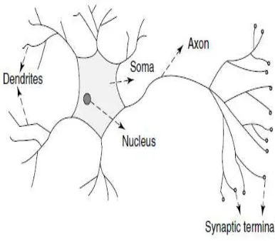
capability for processing the information. The human brain has more than 10 billion interconnected neurons. Each neu-ron in the human brain is a cell which uses the reactions to receive, process, and transmit information. The networks of nerve fibers are called dendrites which are connected to the cell body or soma, where the cell nucleus is located. The axon is a single long fiber extending from the cell body. This axon branches into strands and substrands, to connect to other neurons through synaptic terminals or synapses. The neurons receive signals through synapses. The neurons start to activate and emit a signal through the axons when they receive strong signals, the potential of the signals reach a threshold, a pulse is sent down the axon and the cell is fired. Figure (1) shows the general structure of the neural network feed forward system [23, 24].
Figure 1. The mammalian neuron.
In neural networks, the effects of the synapses are represented by connection weights that modulate the effect of the associated input signals. The transfer function is used to represent the nonlinear characteristic exhibited by neu-rons. The impulse of the neuron is equal to the weighted sum of the input signals that transformed by the transfer function. By adjusting the weights the artificial neuron starts to learn [24]. An artificial neural network is com-monly used for forecasting. As the size of the input data increases, accuracy will increase. The neural network con-sists of one input layer, one output layer and one or more hidden layers. Each layer consists of a number of neurons. In feed forward networks, the signal flow is coming from input to output and there is no feedback connections. In the recurrent networks there is a feedback connection. There are several neural network structures like recurrent or El-man networks, adaptive resonance theory maps, competi-tive networks…., which are used according to the proper-ties and requirements of the application.
The neural network has to be configured to produce the desired set of outputs for a certain set of inputs. There are many methods used to configure the ANN. A common way is to set the weights explicitly by using a priori knowledge.
Another simple way is to train the neural network by feed-ing it teachfeed-ing patterns and allowfeed-ing it to change its weights according to some additional learning rule which is easier but requires additional processing time. The output of each neuron can be expressed as a function of the input signals as:
Yj(t) = f (∑ ) for j = 1,…. H1
Yk(t) = f (∑ ) for k = 1,…. H2
Or(t) = f (∑ ) for r = 1,…. Z
Yj(t) & Yk(t) = Quantity computed by the first and
second hidden neurons respectively. Or(t) = Network output.
X & Z= Number of input and output neurons.
H1 & H2= Number of first and second hidden neurons.
Wij, Wjk & Wkr = Adjustable weights between input and
first hidden layer, the first and second layer and the second and output layer.
bi = Biases.
f = Transfer function.
(a) The general structure of the neural network multi layer feed forward system.
(b) The structure of the model used in this paper.
Figure 2. Neural network structure.
each node, at the output layer. A forward path is used, and the errors are calculated which is the difference between the desired and actual data for each node in the output layer. The errors are used to determine weight changes in the network depending on the learning rule. The backpropaga-tion algorithm, the perceptron rule, and the delta rule are typical supervised learning techniques. In unsupervised learning, the output unit is trained to respond to pattern clusters within the input. The system attempts to discover statistically salient features of the input. Here the system develops its own representations from the input. In rein-forcement learning the system is taught what to do, and how to map situations to distinguish features of reinforce-ment learning. Trial and error search and delayed reward all characterize reinforcement learning. In this approach the learner is not informed which actions to take first for solv-ing a certain problem, but it is informed to discover which actions yield the most reward by trying them [23-27]. There are some rules that should be considered while dealing with ANN like the selection of the raw data patterns for training, the topology of the network, and the training algorithm that has faster convergence properties and lower computational time [25].
A neural network is commonly used for forecasting. As the size of the input data increases accuracy will increase. The neural network consists of one input layer which in our case is the time index and one output which is the tidal speed or the tidal direction and one or more hidden layers. Each layer consists of some neurons. The weight matrices, the number of layers, neurons, epochs of training, inputs and the transfer functions affect on the ANN performance. The back propagation algorithm is an efficient method for changing the weights in a feed forward network, with diffe-rential activation function units and supervised training, to learn a training set of input/output examples. It depends on gradient descent that adjusts the weights to reduce the sys-tem error [28].
Figure (2.a) shows the general structure of the ANN. The system which is used in this paper has only one input and one output as shown in figure (2.b).
3.4. Fourier Series based on Least Square Model Struc-ture (FLSM) [29-31]
The estimated data may be defined using Fourier series as:
! "# $, % &'( ) * + !
"# - % &'( ) * ./&+ % ./& ) * &'(+
Where: DC= Constant value depending on the data (the average value),
K=discrete time, a= amplitude,
i=number of harmonics in the wave,
+= the phase shift. The Fourier series parameters may be
determined using the LSM.
Now let us define the actual data as Z=DC+HX+e(k), e(k)is the error (residuals), then we may apply the least square model as follows to estimate the Fourier series pa-rameters.
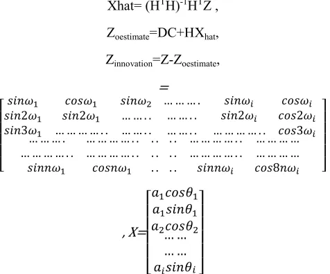
Xhat= (HTH)-1HTZ ,
Zoestimate=DC+HXhat,
Zinnovation=Z-Zoestimate,
= 0 1 1 1 1
2&'(2)&'() &'(2)./&) &'()… … . .
&'(3) … … … … . . … … . .
… … … . &'() ./&)
… … . . &'(2) ./&2)
… … . . … … … … . . ./&3)
… … … . … … … … . . . .
… … … … . . … … … … . . . .
&'(() ./&() . .
. . … … … … . . … … … … . . … … … … . . … … … …
. . &'(() ./&8()
8 9 9 9 9 : , X= 0 1 1 1 1 2% ./&+% &'(+
% ./&+… … … … % &'(+.89
9 9 9 :
H is a matrix that has a number of rows equal to the number of the input data and number of columns depending on the number of harmonic used. X is a resulting vector coming from the matrix H and the input data.
In the following section we will use the FLSM, ANN model and a hybrid of ANN and FLSM for the prediction of the tidal speed during a month. We will use the innovation (residuals) data as the input to the ANN in case of a hybrid model. The data that we used in this paper is a commercial data so we used it after multiplying by a factor and shifting it.
4. Proposed Networks Construction of
the Tidal Current Speed Forecasting
Model
A. ANN model
In this model we use ANN feed forward back propaga-tion for training the proposed model.
B. FLSM Model
In this model we use Fourier series based on the Least Square method for training the proposed model.
C. Hybrid model of FLSM and ANN
describing each step in the hybrid model.
Figure 3. Hybrid model FLSM and ANN flowchart.D. Hybrid model of ANN and FLSM.
This model consists of the tidal current prediction using the ANN at the beginning then find the error between the exact and the predicted data, and this error is called innova-tions. Secondly, we try to use these innovations to feed the FLSM model as an input. Finally the full model is equal to the ANN plus the FLSM. The flowchart shown in figure (4) describing each step in the hybrid model.
Figure 4. Hybrid model of ANN and FLSM flowchart.
5. Tidal Current Data Identifications
(Tidal Speed Models)
5.1. Fourier Series Model based on Least Square Method (FLSM)
In this section we try to use Fourier series based on the least square model for the tidal current prediction. We use the percentage of error (P. E.) for comparing between dif-ferent proposed methods.
The percentage of error (P. E.) = ((ZActual – ZPredicted)/ Z
Ac-tual) *100.
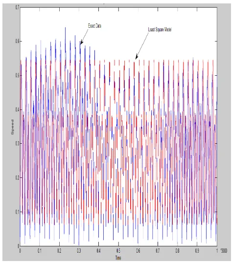
After using the FLSM we find that the percentage of er-ror is 0.6399% for 70% of the data and 0.817 for the other 30% of the data. This means that the error is depending on the number the data and the time that the data taken as its shape will be different from time to time. Figure (5) shows the exact and the estimated data using FLSM for 70% of the available data and figure (6) shows the other 30%. The time for the collected data is measured after each ten mi-nutes and we try to use a code for the time such that the time 1 is the first ten minutes and the time 2 is the second ten minutes and so on till we reach the end. The time on the second graph was measured also at each ten minutes after ten minutes of the end of the first graph. This means that the time on the second graph starting from the 3001*10 minutes which is after ten minutes from the end of the first graph and this means that the time1 on the second graph is equal to 3001*10 minutes for the first graph. The speed in all graphs is in m/s.
Figure 6. The relation between the speed and the time of the tidal currents after using the FLSM for the exact untrained and the estimated data.
5.2. ANN Model
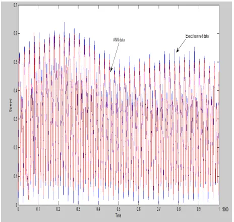
In this section we try to use the ANN for tidal current speed prediction for the same data used in the previous sec-tion. We use the exact data without modifications as an input to the ANN. After 20,000 epochs, 225 neurons in the first layer, the mean squared error became 0.000336. The percentage of error of the trained exact data became 0.3903 and for the estimated data became 3.0946. The exact trained data and the estimated ANN data are plotted in figure (7).
Figure 7. The relation between the speed and the time for the tidal cur-rents after using the predicted ANN and the exact trained data.
The percentage of error for the predicted trained data is very small but for the predicted untrained data is still high. The exact untrained data and the predicted ANN data are
shown in figure (8)
Figure 8. The relation between the speed and the time for the tidal cur-rents after using the predicted ANN and the exact untrained data.
5.3. Hybrid model of FLSM and ANN
The models used in the case of FLSM and ANN give a high percentage of error for the predicted not trained data so we will try to use a hybrid of FLSm and ANN. In the hybrid model we try to find the innovation data using FLSM and use this innovation as an input to the ANN. After 20,000 epoch, 225 neurons in the first layer, i=6, the mean squared error became 0.000380. The percentage of error for the innovation of the trained exact data is 0.1304.
The exact trained data and the predicted from the hybrid model have a percentage of error of 0.3328 and is shown in figure (10). The exact not trained data and the predicted ANN from the hybrid model is shown in figure (10). The predicted ANN from the hybrid model has a percentage of error of 0.4737.
Figure 10. The relation between the speed and the time for the tidal cur-rents after using the hybrid model of FLSm and ANN and the exact un-trained data.
5.4. Hybrid model of ANN and FLSM
This model is the same as the previous model except the order. So the data is fed to ANN and then find the innovation data. After that use the innovation data to feed FLSM. The exact trained data and the predicted from the hybrid model has a percentage of error of 0.357 for the trained set of data and 0.672 for the untrained data.
We can summarize the previous analysis in table (1). We conclude that the percentage of error for the hybrid model of FLSM and ANN is the smallest value in the case of the trained or predicted data. So these models can be ranked as follows in terms of high accuracy:
a. Hybrid of FLSM and ANN. b. Hybrid of ANN and FLSM. c. FLSM.
d. ANN.
As the number of data points increased and included all changes the error will be decreased. In the next section we try to use the same algorithms for another set of data (the direction magnitude forecasting) to prove the validity of the proposed model.
Table 1. Comparison between different used models for tidal current speed forecasting.
Comparison between different used models
Type of comparison ANN FLSM FLSM
+ ANN
ANN + FLSM
% Error of trained
data (70%) 0.3903 0.6399 0.3328 0.357
% Error of
forecasted data (30%) 3.0946 0. 817 0.4737 0.672
6. Validation of the Proposed Models
(Tidal Direction Forecasting)
In this section we try to apply the proposed algorithms to forecast the direction magnitude of the tidal current.
6.1. Fourier Series Model based on Least Square Method
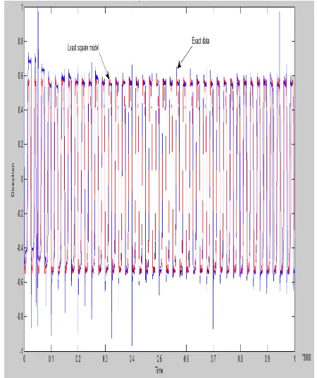
We use the FLSM for the tidal direction for the same pe-riod and the site that was used for the speed forecasting. Fourier series based on the least square model data and the exact data are drawn in the same graph as shown in figure (11) for 70% of the whole data and in figure (12) for 30% of the whole data. The percentage of the error for 70% of the whole data is equal to 0.7339 and for the other 30% is equal to 0.861. The direction in all graphs is in degree.
Figure 12. The relation between the direction and the time of the tidal currents after using the FLSM and the exact data untrained data.
6.2. ANN Model
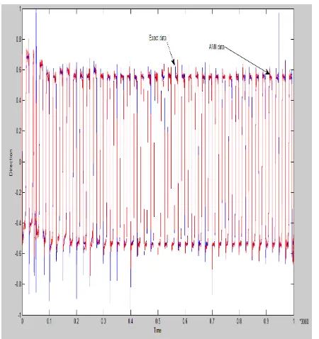
We use the direction magnitude data as an input to the ANN without any modifications and training the ANN for 20000 epochs, 225 neurons in the first layer, the mean squared error became 0.000579. The percentage of error for the trained data is 0.5169 and for the estimated data is 3.8496. The exact trained data and the predicted ANN data are plotted in figure (13) and the exact untrained data and the predicted ANN are shown in figure (14). The percen-tage of error in the untrained predicted data is still high so we use the hybrid of ANN and FLSM.
Figure 13. The relation between the direction and the time for the tidal currents after using the predicted ANN data and the exact trained data.
Figure 14. The relation between the direction and the time for the tidal currents after using the predicted ANN data and the exact untrained data.
6.3. Hybrid model of FLSM and ANN
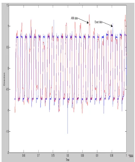
As described in the previous section this hybrid model consists of the FLSM and ANN. We use FLSM to predict the tidal current direction magnitude and then calculate the innovations which is the difference between FLSM and the exact data. The innovations are fed to the ANN as an input. We then add the innovations to FLSM to find the whole model. The mean squared error for the innovations is 0.000679. Figure (15) shows the trained data versus the hybrid. The percentage of error for this model is equal to 0.1169 for the trained data. Figure (16) shows the predicted data versus the hybrid data for the untrained period of data. The percentage error for untrained data is equal to 0.4970.
Figure 16. The relation between the direction and the time for the tidal currents after using the hybrid model and the exact untrained data. 6.4. Hybrid model of ANN and FLSM
This model again is the same as the previous model ex-cept the order. So the data is fed to ANN and then the inno-vation data is fed to FLSM. The exact trained data and the predicted from the hybrid model has a percentage of error of 0.156 for the trained set of data and 0.675 for the un-trained data.
We can summarize the previous analysis in table (2). We find that the hybrid model of FLSM and ANN has the smal-lest error.
Table 2. Comparison between different used models for tidal current direc-tion forecasting.
Comparison between different used models
Type of comparison ANN FLSM FLSM
+ ANN ANN + FLSM
% Error of trained
data (70%) 0.5169 0.7339 0.1169 0.156
% Error of forecasted
data (30%) 3.9892 0.917 0.4970 0.675
7. Conclusion
Four models are proposed in this paper for tidal current speed and direction magnitude forecasting. Using either FLSM or ANN alone for the prediction of tidal current Speed and direction is not recommended. The models are ranked from the highest accurate to the lowest accurate. The hybrid of FLSM and ANN is the best model for the tidal current speed forecasting model and has a high
accu-racy. The hybrid of ANN and FLSM is the next best model. Then FLSM and ANN at the end. In this paper we use the proposed model for the speed forecasting of the tidal cur-rent and the model gives good results. We validated this work by applying the proposed algorithms for another set of data (tidal current direction magnitude) and the simu-lated results show better performance after using the hybrid model of FLSM and ANN. This is because we add the ad-vantages of FLSM and ANN at the same time to be in one model.
References
[1] “Tidal Stream” Available online (November 2010), http://www.tidalstream.co.uk/html/background.html.
[2] “Marine Current Turbines” Available online (October 2010), http://peswiki.com/index.php/Directory:Marine_Current_Tu rbines_Ltd#How_it_Works.
[3] Darwin, G.H., on an apparatus for facilitating the reduction of tidal observations. Proceedings of the Royal Society, Se-ries A 52, 345–376, 1892; Available at: http://archive.org/details/philtrans02858224.
[4] Doodson, A. T., The Harmonic Development of the Tide-generating Potential, Proc. Roy. Soc., London, pp 305-329,
1923. Available at:
http://archive.org/details/philtrans08044568.
[5] Doodson, A.T., The analysis and predictions of tides in shal-low water. International Hydrographic Review: Monaco 33, 85–126, 1958.
[6] John, V. “Harmonic tidal current constituents of the Western Arabian Gulf from moored current measurements.” Coastal Engineering, Vol. 17,pp. 145–151, 1992.
[7] French, M. N. , Krajewski, W. F. & Cuykendall, R. R. “Rainfall forecasting in space and time using a neural net-work”, Journal of Hydrological Sciences, 1992.
[8] Raman, H. & Sunilkumar, N. “Multivariate modeling of water resources time series using artificial neural networks”, Journal of Hydrological Sciences, pp. 145 - 163, 1995.
[9] Christian Dawson & Robert Wilby “An artificial neural network approach to rainfall- runoff modelling”, Journal of Hydrological Sciences, pp. 47- 66, 1988.
[10] Coulibaly, P., Anctil, F., and Bobee, B.: Daily reservoir in-flow forecasting using artificial neural networks with stopped training approach,Journal of Hydrological Sciences, pp. 244–257, 2000.
[11] T.L. Lee, and D.S. Jeng “Application of Artificial Neural Networks in Tide Forecasting”, Journal of Ocean Engineer-ing, Vol. 29, No. 9, pp. 1003-1022, August 2002.
[12] M. Campolo, A. Soldati and P. Andreussi, , “Artificial neur-al network approach to flood forecasting in the river Arno”, Journal of Hydrological Sciences, 2003.
[14] Lee, T. L., C. P. Tsai and R. J. Shieh “Applied the Back-propagation Neural Network to Predict Long-Term Tidal Level” Asian Journal of Information Technology, Volume 5, Issue 4, pp. 396-401, 2006.
[15] Ritu Vijay, and Rekha Govil “Tidal Data Analysis using ANN”, Journal of World Academy of Science Engineering and Technology, 2006.
[16] Bang-Fuh Chen, Han-Der Wang, Chih-Chun Chu “ Wavelet and artificial neural network analyses of tide forecasting and supplement of tides around Taiwan and South China Sea”, Journal of Ocean Engineering, Vol. 34, Issue 16, pp. 2161-2175, November 2007.
[17] Jan F. Adamowski “River flow forecasting using wavelet and cross-wavelet transform models” Journal of Hydrologi-cal Processes, Volume 22, Number 25, pp. 4877–4891, 2008.
[18] Remya, P.G., Kumar, Raj, and Basu Sujit, “Forecasting Tidal from Tidal levels using genetic algorithm”; Journal of Ocean Engineering, Volume 40, pp. 62-68, February 2012.
[19] Burrage, D.M., C. R. Steinberg and K.P. Black “Predicting long-term currents in the Great Barrier Reef”, 11th Australa-sian Conference on Coastal and Ocean Engineering, Austral-ia, 1993.
[20] William Mendenhall, Terry Sincich A Second Course in Statistics: Regression Analysis, Amazon, 2011.
[21] Golberg, M. , Cho, H. A. “Introduction to Regression Analy-sis” , Southampton : Wit Press, 2003.
[22] Rahman, S., Bhatnagar, R. “An expert system based algo-rithm for short term load forecast”,IEEE Transaction on Power Systems, Volume 3, Page(s): 392 – 399, 1988.
[23] Hamed H. H. Aly, and M. E. El-Hawary, “A Proposed ANN and FLSM Hybrid Model for Tidal Current Magnitude and Direction Forecasting” accepted at the IEEE Journal of Ocean Engineering, 2013.
[24] S. A. Soliman ; A. M. Al-Kandaria; and M. E. El-Hawary ”Time Domain Estimation Techniques for Harmon-ic Load Models” Journal of ElectrHarmon-ic Power Components and Systems, Volume 33, Number 10, 2005.
[25] “Artificial Neural Networks” available online (August 2012), http://www.softcomputing.net/ann_chapter.pdf
[26] Zurada, J., “Introduction to Neural Systems”, West Publish-ing, 1992.
[27] Ma L., Khorasani K. “New Training Strategies for Construc-tive Neural Networks with Application to Regression Prob-lems” Neural Networks, Vol. 17, No. 4, May 2004.
[28] T. Q. D. Khoa, L. M. Phuong, P.T.T.B inh, N. T. H. Lien “Application of Wavelet and Neural Network to Long-Term Load Forecasting” International Conference on Power Sys-tem Technology , Singapore, 21-24 November 2004.
[29] S. A. Soliman; A. M. Al-Kandaria; and M. E. El-Hawary ”Time Domain Estimation Techniques for Harmon-ic Load Models” Journal of ElectrHarmon-ic Power Components and Systems, Volume 33, Number 10, 2005.
[30] Atif S. Debs, “Modern Power Systems Control and Opera-tion” Boston, Mass.: Kluwer Academic Publishers, 1988.