The Design of Curved Endwall with Leading-edge Deformation

http://www.sciencepublishinggroup.com/j/ijepe doi: 10.11648/j.ijepe.20200901.11

ISSN: 2326-957X (Print); ISSN: 2326-960X (Online)

The Design of Curved Endwall with Leading-edge

Deformation

Zhang Xuyang

CSIC 704 Research Institute, Shanghai, China

Email address:

To cite this article:

Zhang Xuyang. The Design of Curved Endwall with Leading-edge Deformation. International Journal of Energy and Power Engineering.

Vol. 9, No. 1, 2020, pp. 1-10. doi: 10.11648/j.ijepe.20200901.11

Received: December 22, 2019; Accepted: December 30, 2019; Published: January 27, 2020

Abstract:

The inlet boundary layer separates in front of the leading edge of the blade on the endwall and forms the pressure side leg of horseshoe vortex and the suction side one. The pressure side leg of the horseshoe vortex immediately moves toward to the suction side and form a stronger vortex, ”passage vortex”, in the cascade. These vortices mentioned above are called secondary flows which will result in an increase of secondary flow losses and a reduction of stage efficiency. In this paper, the flow characteristics are analyzed in the leading edge region and inside the cascade based on the numerical simulation results of the Langston cascade. A new type endwall design method, curved endwall structure combined with the deformation in the leading edge region, is established and optimized. It can be observed that the new structure can efficiently reduce the strength of the horseshoe vortex and suppress the generation of the leading edge separation line and saddle point. The uses of the new structure also decrease the pressure gradient between the pressure side and the suction side in the streamline direction, which suppresses the deviation of the pressure side horseshoe vortex from the pressure side of the endwall to the suction side and delays the formation position of the passage vortex. The rate of increase in the total pressure loss coefficient along the mainstream direction also decreases 25.34% in the exit of the cascade.

Keywords:

NURBS, Secondary Flow, Leading-edge Position, Curved Endwall

1. Introduction

In the endwall region of turbine cascade, the flow is strongly three dimensional and has significant components normal to the designated streamwise velocity. The difference between actual endwall flow and the inviscid midspan flow forms a vortex above the endwall. It moves through, entrains more fluid and leaves the cascade in a large passage vortex. It dissipates the main flow energy and may account for 30%- 50% of the total loss [1] in a low aspect turbine cascade. In addition, the exit flow angle in the endwall region is over or under turned, which generates an extra incidence loss on the downstream blade row.

Langston [2], Goldstein [3] and Wang et al [4] have described the structure of secondary flow with a series of complex vortices structure. Although their detailed structures are slightly different, their model have some common features. The upstream flow boundary layer separates at the blade leading edge and separates into two branches, the pressure side leg of horseshoe vortex (HPV) and the suction side leg of

horseshoe vortex (HSV). When the HPV moves through the flow channel, it starts at the leading edge in the pressure side and leaves at the trailing edge in the suction side. The blade-to-blade (BTB) pressure gradient pushes the HPV across the cascade from the pressure side to the suction side. At the exit plane, HPV gets merged with HSV and forms a passage vortex (PV). Denton’s [5] reveals that the PV strength is proportional with the endwall loss. Therefore, one of the flow control methods to reduce endwall losses is to modify the geometries of blade hub section including airfoil and hub surface, which intends to alleviate the BTB pressure gradient so as to low the strength of the PV.

strength of corner vortex, weaken the strength of the passage vortex and reduce the loss of the secondary flow of the cascade by 47%. Through the simulation, Shih and Lin [8] further explained that the decrease of velocity and velocity gradient caused by the use of fillet reduce the intensity of turbulence and the aerodynamic performance of the cascade is improved. Wei [9] used a water-drop shaped fillet extending downstream in the endwall region which causing the disappearance of local pressure fluctuation on the stator surface. Sangston [10] and Lyall [11] designs the fillet in the leading edge region to change the inlet angle near endwall the loss of endwall loss by 20%.

Non-axisymmetric endwall (NAEW), which is also called curved endwall, is also often used in the turbine passage. Atkins [12] proposed an idea of contoured hub surface to accelerate or decelerate local flow to control the endwall pressure distribution in 1984. It is then developed on an annual cascade and named as non-axisymmetric endwall. A lot of

researches on turbine cascades have proven that

non-axisymmetric endwall efficiently decreases the strength of secondary vortex, reduces the loss of secondary flow and controls the wall heat transfer on the endwall. Mahesh [13], Saha [14], Taremi [15] designed their own NAEW for the stator vanes and reduce the BTB pressure gradient, the exit flow deviation and total pressure loss. Secondary flow loss measured at the exit of the cascade is obviously decreased. Rose [16], Zimmermann [17], Bergh [18] designed the NAEW for rotor blades, which increase the cascade efficient by 0.51%-4.6%. Their study results also show that the use of non-axisymmetric endwalls in the rotor cascades have potentials to improve the inlet flow of next stator row. Lynch [19] and Mensch [20] construct NAEW configurations to investigate the influence of its effects on heat transfer. Local heat transfer coefficients at part NAEW surface are shown to be lower than at normal flat surface. Secondary loss caused by the film cooling on the endwall are also restrained.

Nowadays, fillet structure and curved endwall structure have been studied in detail both at home and abroad. In order to have a better control effect on the secondary flow in the flow channel, predecessors used to combine them together to form the new structure [21-23]. Although the above research has achieved good flow effect, the simple superposition of fillet and curved endwall also forms more complicated structure, which brings more difficulties for machining. This paper attempts to solve a problem by building a new structure, Curved Endwall with Leading-edge Deformation (CELD), which containing both fillet and curved endwall’s effects. In this paper, Langston blade shape is used as the research object. Numerical method are used to have a detailed research about the influence of CELD structure on the flow in the endwall region. The simulation result of CELD structure is compared with the curved endwall structure and the original model.

2. Computational Methodology

In this paper, Langston turbine cascade is built based on the experiment of Graziani [24]. The leaf shape data is shown in

Table 1. Langston turbine cascade is a low speed, large curved and high load cascade. The horseshoe vortex and passage vortex inside the flow channel is strong and can be easily observed. Based on its upon character, Sieverding [25], Holley [26] and others use Langston turbine cascade as an experimental and simulation analysis object.

Table 1. Cascade Geometry.

Parameter Value

Axial chord length 281.3mm Chord length/axial chord length 1.22

Relative pitch 0.96

Aspect ratio 0.99

Inlet angle 44.6°

Exit angle 26°

Commercial software are used in this article to complete the numerical calculation of original model and model with curved endwall. Steady Reynolds averaged navier-stokes equation (RANS) is used in simulation computation. Both turbulent and energy equations are solved by using second-order accuracy. The turbulence model uses Shear Stress Transport (SST). The simulation results obtained by using this turbulent model meet well with the experimental results.

In order to accurately simulate the flow structure of the leading edge of the cascade, an entrance domain which length equals the axial chord length is constructed before the blade domain. Inside the blade domain, a length equals 0.5 times axial chord length is also exists in the front side of the blade. Refer to the Grazinai’s experiment, the boundary conditions is shown in Table 2. The velocity inlet with turbulence and temperature is given in the inlet of the computational domain. The top surface is set as the symmetric boundary conditions. The faces on the both sides is set as periodic boundary. Static pressure is given in the exit of the computational domain. The endwall and blade are set as constant heat flux boundary conditions. A calculation domain which length equals 0.5 times axial chord length is given behind the blade in the blade domain. And an exit domain, which is one time axial chord length long, is set behind the blade domain.

Table 2. Test Condition [24].

Parameter Value

Boundary layer thickness 3.3cm Leaf surface heat flux 1310W/m2 Endwall surface heat flux 1830W/m2

Inlet velocity 34m/s

Mainstream turbulence 1% Inlet Reynolds number 5.5×105 Mainstream temperature 300K

Outlet pressure 101.3KPa

Commercial grid-building software is used in this article to draw structured grids for the calculation domain. In order to meet the requirements of grid independence, five gradually encrypted

grid from 7.35×105 grid number to 3.67×106 are used to calculate

the Langston turbine cascade for mass flow and static pressure efficient, as shown in Figure 1. When the number of grids

reaches 2.32×106, the calculation results do not change with the

independence requirements. After considering the calculation accuracy and calculation time comprehensively, this grids is used in the simulation calculation.

Figure 1. Independence verification of mesh number.

The number of grids we used in this article is 2.32×106. The

grid is fined at the proximal wall position. The thickness of the first layer of the proximal wall is 0.012 mm. Yplus of the endwall and blade is less than 1. The grid meets computational needs. Figure 2 shows the grid distribution of the original model. The O-type grid is used around the cascade and the H-type grid is used in the middle of the flow channel. The thickness of the first layer of the grid of the O-grid on the surface of the blade is 0.012mm, and the increasing rate of the grid is 1.1. The number of circumferential nodes in the calculation domain is 108, 196 in the axial direction and 100 in the radial direction. The calculated residuals of each

equation are less than 10-6. In the 500 iterations, the change of

the mass flow at the outlet is less than 0.1%, and the calculation results converge.

(a) Grid topology.

(b) The mesh of the leading edge and tailing edge.

Figure 2. Depictions of the computational domain.

The static pressure coefficient at the 50% blade height from the experiment [26] and the simulation are shown in Figure 3. The calculated values are basically consistent with the experimental values.

The formula of the static pressure coefficient is as followed:

0 *

0 0

p

P P

C

P P

− =

− (1)

In this formula, P is the local static pressure, *

0

P is the inlet

total pressure, P0 is the inlet static pressure.

Figure 3. Measured and predicted blade surface static pressure at mid-span.

3. Curved Endwall Design and Results

3.1. Design Process

Curved endwall contouring used in this paper is accomplished by four steps. First step is to determine the fixed point and the controllable point on the endwall according to the limit streamline distribution on the endwall of original model. Secondly, the pressure distribution at each control point was extracted. Thirdly, calculate the relative lifting height of each control point by using the equation which establishes the relationship between distribution of pressure and the uplift height by using Mass Conservation Equation and Bernoulli Equation. Fourth, Use these control points to construct curved endwall. The method to build the curved endwall is similar to Schobeiri [27], but not exactly the same. The feasibility and rationality of this method has proved in detail in that paper. Therefore, it is feasible to use this method to construct the curved endwall in the prior research.

3.2. Design Results

The contours of the designed curved endwall are shown in Figure 4. The figure clearly shows the lifting of the pressure side of the endwall and the drop of the suction side.

on the pressure side leg of horseshoe vortex to the suction side and delay the formation of the passage vortex.

Figure 4. Contours of the endwall height.

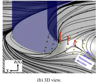
Figure 5 displays the 3D streamline near the endwall colored in red, limiting streamline on the endwall colored in black and Q criterion number isosurface equals 150000 by using blue transparent surface.

As shown in Figure 5 (a), when the endwall boundary layer approaches the leading edge of the blade, it separate in a three-dimensional manner and turn into pressure side and suction side horseshoe vortex. Due to the strong pressure gradient between pressure side and suction side of the blade, the pressure leg of the horseshoe vortex immediately moves toward the suction side after it enters the passage and directly lead to the generation of the passage vortex.

After using the curved endwall, it can be noticed that the deviation of the pressure side leg of horseshoe vortex toward the suction side is suppressed after it generates. The pressure side leg of horseshoe vortex is closer to the pressure side of the endwall compared with the original model.

(a) Original model.

(b) Model with Curved Endwall.

Figure 5. Flow topology in the cascade with Q-criterion number，limiting

streamline on the endwall and streamline in the cascade.

Although the curved endwall has a good control effect on the deviation of the horseshoe vortex in the cascade, its flow structure in the leading edge endwall region is similar to the original model. The distribution of limiting streamline of the original model and curved endwall model is shown in Figure 6. The saddle point and the leading edge stagnation point are signed on the endwall as red points. Boundary layer separation line are signed as blue line.

It can be observed from the Figure 6 (a) that the limiting streamline on the both side of the separation line close to it. The direction of limiting streamline between the saddle point and the leading edge stagnation point is opposite to the mainstream direction, which causes the low energy fluid to roll up in this region and form a stronger horseshoe vortex. The reverse flow region between the saddle point and leading edge stagnation point is the fundamental cause of the horseshoe vortex.

After using the curved endwall, the position of the saddle point and the streamline moving downstream, as shown in Figure 6 (b). But the basic flow structure has not changed. The saddle point and reverse flow region still exists.

(a) Original model.

(b) Model with curved endwall.

Figure 6. Limiting streamline on endwall.

4. Deformation in the Leading Edge

Region

After comprehensive consideration, this paper decided to describe the new endwall modeling with non-uniform rational B-spline surfaces (NURBS). Compared with other surface configuration methods, the NURBS configuration method has the characteristics of simple parameterization, large design space and continuous surface curvature. The use of NURBS in this paper builds a clear relationship between control point locations and surfaces.

NURBS surface is a bivariate piecewise rational function with P orders in u direction and q orders in v direction:

, , , , 0 0 , , , 0 0 ( ) ( ) ( , ) ( ) ( ) n m

i p j q i j i j i j

n m

i p j q i j i j

N u N v w P

S u v

N u N v w

= =

= =

=∑ ∑

∑ ∑

0≤u v, ≤1 ₍₂₎

, i j

P _{is represent of the control point, and the number of}

points are (m+1) and (n+1) in u and v direction respectively.

,

{wi j} is a weight factor, {Ni p, ( )}u and {Nj q,( )}u are the basic

functions of non-rational B spline based on the vector U and

V. Changing the values of {wi j,} and {Pi j,} can adjust the

shape of the surface accurately.

The leading-edge deformation is controlled by 6×5 control points matrix on the curved endwall, as shown in Figure 7. The control points matrix in this paper is built based on the leading edge stagnation point and saddle point, whose lift distance are the control variables. The adjoint uplift point which is colored in blue change its height with the saddle point and stagnation point. The height of other control points, expect leading edge point and saddle point, does not change in this study. It is expected that forming the leading-edge deformation by changing the height of these control points can be the most effectively way to improve the flow in the leading edge, which can divert the low energy stagnation fluid away from the leading edge. The curved endwall with leading edge deformation is also abbreviated as CELD in the following section.

Each control point is given a certain variation region to avoid irrational design caused by excessive changes of the control point and to reduce the amount of optimization calculations. The lifting range of the leading edge stagnation

point is controlled at [5, 20] (mm) (δ to 4δ ). The lifting

range of the saddle point is controlled at [2.5, 7.5](mm) (0.5δ

to 1.5δ ). The shape of the endwall can be accurately and

clearly defined by changing the lifting distance of the control point relative to the original curved endwall model. For example, “5-10 CELD” represents the leading-edge deformation is formed by the saddle pointlifting 5 millimeter and the leading edge stagnation point lifting 10 millimeter.

(a) Top view.

(b) 3D view.

Figure 7. Contoured surface control point placement in the leading edge.

5. Optimization Method and Result

In this paper, the aerodynamic optimization design method based on Kriging surrogate model is used to optimize the design of the new endwall. The design flow chart is presented in Figure 8. The lifting distance of saddle point and stagnation point are treated as the design variable. Initial sample set is built by changing the design variable. Commercial Fluid Mechanics Software is used to calculate the flow field and to obtain the value of the evaluation index. Kriging surrogate model is used to build an approximte model between design variable and evaluation index. If the difference of the objectives functions between two rounds of optimization is larger than 0.1%, optimization process won’t be treated as converge. The simulation results will be added to the sample library to start another optimization cycle. Repeat the above steps until convergence. The method involves experimental design, numerical calculation and

optimization methods. Compared with the global

optimization algorithm, the use of the surrogate model reduces the workload of the optimization calculation and has a higher efficiency and turns to be a better method.

The total pressure loss coefficient of the cascade is treated as an evaluation index in this paper. The formula of the total pressure loss coefficient are as followed:

2 1 2 to t pt P P C u ρ − = (3)

In this formula, Pto represents the total pressure of the inlet,

t

P represents the total pressure of the outlet and

u

represents the velocity of the inlet.

Through two rounds of optimization, the difference between the evaluation indicators of the two rounds’ optimization results is lower than 0.1%. Optimal calculation results are convergent. The final result of the optimization calculation is that the saddle point rise 4.2mm and the stagnation point rise 10.85mm and the curved endwall with leading deformation is called “4.2-10.85 CELD”. After using

this endwall, the value of Cpt achieve to its minimum value

initial sample set, the yellow cube represent the optimization results of the first two rounds and the red pentagon is the final result, “4.2-10.85 CELD”, after the optimization. The x-coordinates is the lifting distance of leading edge stagnation point. The y-coordinates is the lifting distance of

saddle point. The z-coordinates is the value of Cpt.

Figure 8. Flowchart for the adaptive optimization method.

Figure 9. The response surface as a function of the lifting distance of the

saddle point and the stagnation point with twelve initial sample points.

6. Results and Discussions

The contours of the optimized endwall structure, “4.2-10.85 CELD”, are shown in Figure 10. Figure 10 depicts the three-dimensional view of the leading edge of the endwall that clearly shows the endwall deformation at that position compared with the original curved endwall model.

Figure 10. Contours of the end-wall heightandthree-dimensional view of the

endwall in the leading edge.

The use of “4.2-10.85 CELD” can effectively suppress the generation of the saddle point, separation line and reverse flow region.

Figure 11 displays the distribution of endwall limiting streamline of “4.2-10.85 CELD”. The original saddle point from original model and the leading edge stagnation point are signed in the figure as red point. Separation line is also signed on the endwall as blue line. The saddle point in the figure has already marked in Figure 6 (a).

“4.2-10.85 CELD” improves the flow in the leading edge by deforming the endwall between the saddle point and leading edge stagnation point, suppressing the generation of secondary flow. Compared with the original model and the curved endwall model, saddle point can not be observed and the position of separation line move downstream significantly on the endwall of “4.2-10.85 CELD”. The whole leading edge reverse flow region disappears. The stagnation fluid at the leading edge position is effectively dredged.

Figure 11. Limiting streamline on endwall of CELD model.

The guiding of the leading edge stagnation fluid also effectively suppresses the strength of the horseshoe vortex in the leading edge.

Figure 12 displays the distribution of Turbulent Kinetic Energy (TKE) in the leading edge of “4.2-10.85 CELD”. Comparing with Figure 12 (a) and Figure 12 (b), it can be found that since the fluid in the mainstream boundary layer is no longer rolled up in the leading edge, but is guided by the end wall to both sides of the leading edge, the strength of the horseshoe vortex at the leading edge position is obviously decrease, the strength of the suction side leg of horseshoe vortex and the pressure side leg of horseshoe vortex are also reduced. Compared with the model only use curved endwall, the “4.2-10.85 CELD” have better effect on the strength of horseshoe vortex controlling. The streamline distribution is also more uniform.

(b) Original CW model.

(c) CELD model.

Figure 12. Streamlines approaching the leading edge and the distribution of

turbulent kinetic energy in the leading edge, showing the generation of horseshoe vortices.

The decrease of the strength of the horseshoe vortex at the leading edge causes the reduce of the secondary vortex strength downstream.

Figure 13 (a) first shows the whole development of the main secondary vortex system of the original model in the endwall region. After the horseshoe vortex forms in the leading edge, it develops downstream and forms pressure side leg and suction side leg. The pressure side leg of horseshoe vortex entrains a majority of the low-momentum, high-vorticity endwall boundary layer moves toward to the suction side under the action of lateral pressure gradient, merges with the suction side leg and grows to form the passage vortex. The secondary vortices mentioned before, two legs of horseshoe vortex and the passage vortex, are signed inside the Figure 13 (a) by using arrow.

Figure 13 (b) (c) (d) displays the distribution of the TKE of the original model in the endwall region at different streamwise position, includingx/Cax=0.2,0.7,1.1. In these figure,

the strength and the position of the secondary vortices can be gotten through the above-mentioned position. They are also respectively indicated on these cloud chart.

Figure 13 (e) (f) (g) displays the distribution of the TKE of the model with curved endwall in the endwall region. It can be observed from the figure that the use of the curved endwall

reduces the strength of the horseshoe vortex at x/Cax=0.2, and

the pressure side horseshoe vortex is closer to the pressure surface compared with the original model. The mergence of the horseshoe vortex and the formation of the passage vortex are restrained by the use of the curved endwall which can be

observed atx/Cax=0.7. The strength of the passage vortex is

reduced by 45.458% compared to the original model at

x/Cax=1.1, and the height of the passage vortex is also slightly

lower than the original model.

Figure 13 (h) (i) (j) displays the distribution of the TKE of the “4.2-10.85 CELD”. It can be noticed from the figure that the position of the horseshoe vortices is similar to the model with curved endwall model, while the strength of the vortices is smaller. The passage vortex generated from the horseshoe

vortices as displayed in x/Cax=1.1 is also significantly affected.

The value of the passage vortex is reduced by 52.02% compared to the original model.

The “4.2-10.85 CELD”structure controls the strength of the horseshoe vortex in the leading edge, which restrains the strength of the each vortex downstream. The strength of the secondary flow structure decreases and the flow at the endwall region is improved.

(a) The distribution of TKE in the flow direction.

(b) x /Cax=0.2 in the original model.

(c) x /Cax=0.7 in the original model.

(e) x /Cax=0.2 in the model with curved endwall.

(f) x /Cax=0.7 in the model with curved endwall.

(g) x /Cax=1.1 in the model with curved endwall.

(h) x /Cax=0.2 in the CELD.

(i) x /Cax=0.7 in the CELD.

(j) x /Cax=1.1 in the CELD.

Figure 13. The flood of Turbulent kinetic energy at different axial cord.

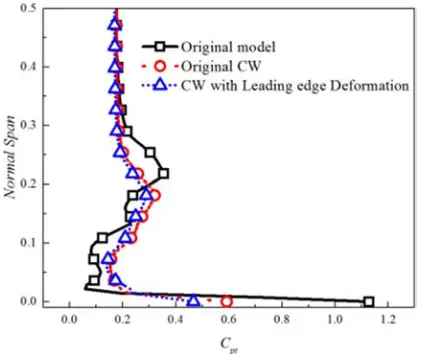
The radial distribution of Cpt in Figure 14 confirms that a

total pressure loss high region occurs at 20% blade height position. This position is corresponding to passage vortex’s location as shown in Figure 13. It also can be noticed that the use of the “4.2-10.85 CELD” reduces the maximum value of total pressure loss coefficient compared with the original model and the model only with the curved endwall. The position of the maximum value also closer to the endwall compared with the original model which has also be mentioned before.

Figure 14. Pitch averaged total pressure loss coefficient at.x/Cax=1.0_.

Figure 15 shows the variation of the total pressure loss coefficient along the flow direction inside the cascade. The total pressure loss coefficient gradually increases monotonically along the flow direction. After using the curved endwall model, the secondary flow loss coefficient’s increase is suppressed due to the decrease of the strength of the secondary vortices. However, after using “4.2-10.85 CELD”, the formation of the horseshoe vortex at the leading edge is controlled, which also leads to the decrease of total pressure loss coefficient along the flow

direction in the position x /Cax=0 . Compared with the

original model, the total pressure loss coefficient decreased by 25.34% and 14.14% lower compared with the model only with curved endwall.

7. Conclusion

The existence of secondary vortex system including horseshoe vortex and passage vortex increase the flow loss of the cascade, decrease the work ability and make the flow condition worse. In this paper, the NURBS is used for the endwall deformation in the leading edge position of the endwall based on the model with curved endwall. Kriging surrogate model then used to optimizate the endwall and obtain the best endwall, “4.2-10.85CELD”(Curved Endwall with Leading-edge Deformation). The use of this structure controls the generation of the horseshoe vortex, moves back the generation of the passage vortex and reduces the total pressure loss coefficient by 25.34%.

The mainstream boundary layer is guided to two sides of the leading edge by the use of the endwall deformation in the leading edge position instead of rolls up and leads to a strong horseshoe vortex. The leading edge saddle point disappears, the separation line moves backward, the leading edge reverse flow region behind the separation line disappears, the formation of the horseshoe vortex at the leading edge position is suppressed and its strength decreases. The pressure side leg of the horseshoe vortex quickly moves toward the suction side due to the strong pressure gradient after it enters the passage, merges with suction side one and form the passage vortex. Due to the use of the curved endwall, the deviation of the pressure side leg of the horseshoe vortex is suppressed, which also moves back the generation position of the passage vortex. The increase in total pressure loss due to the passage vortex is also suppressed. The strength of the passage vortex at the exit position of the cascade is reduced by 45.458%.

The curved endwall model combined the deformation of the endwall in the leading edge position plays a good role in controlling the formation and development of the horseshoe vortex and passage vortex. However, further optimization of the endwall structure and its control of unsteady secondary flow under complex flow condition requires further research. Following research is focused on the further optimization of the curved endwall and the fusion of the complex curved endwall surface with the blade and its effectiveness.

References

[1] SHARMA O P, BUTLER T L. Predictions of Endwall Losses and Secondary Flows in Axial Flow Turbine Cascades [J]. Journal of Turbomachinery, 1986, 109 (2): 229.

[2] LANGSTON L S. Crossflows in a Turbine Cascade Passage [J]. Journal of Engineering for Gas Turbines & Power, 1980, 102 (4): 866.

[3] GOLDSTEIN R J, SPORES R A. Turbulent Transport on the Endwall in the Region Between Adjacent Turbine Blades [J]. Journal of Heat Transfer, 1988, 110 (4a): 862.

[4] WANG H P, OLSON S J, GOLDSTEIN R J, et al. Flow Visualization in a Linear Turbine Cascade of High Performance Turbine Blades [J]. Journal of Turbomachinery, 1995, 119 (1): 1-8.

[5] DENTON J D, DENTON J D. Loss Mechanisms in Turbomachines [J]. Journal of Turbomachinery, 1993, 115: 4 (4): V002T14A1.

[6] ZESS G A, THOLE K A, ZESS G A. Computational Design and Experimental Evaluation of Using a Leading Edge Fillet on a Gas Turbine Vane [J]. Journal of Turbomachinery, 2002, 124 (2): 167-75.

[7] SAUER H, MÜLLER R, VOGELER K. Reduction of Secondary Flow Losses in Turbine Cascades by Leading Edge Modifications at the Endwall [J]. Journal of Turbomachinery, 2001, 123 (2): 207-13.

[8] SHIH T I P, LIN Y L. Controlling Secondary-Flow Structure by Leading-Edge Airfoil Fillet and Inlet Swirl to Reduce Aerodynamic Loss and Surface Heat Transfer [J]. Journal of Turbomachinery, 2003, 125 (1): 48-56.

[9] WEI Z J, QIAO W Y, LIU J, et al. Reduction of endwall secondary flow losses with leading-edge fillet in a highly loaded low-pressure turbine [J]. Proceedings of the Institution of Mechanical Engineers Part A Journal of Power & Energy, 2016, 230 (2).

[10] SANGSTON K, LITTLE J, LYALL M E, et al. End Wall Loss Reduction of High Lift Low Pressure Turbine Airfoils Using Profile Contouring—Part II: Validation; proceedings of the ASME Turbo Expo 2013: Turbine Technical Conference and Exposition, F, 2014 [C].

[11] LYALL M E, KING P I, CLARK J P, et al. Endwall Loss Reduction of High Lift Low Pressure Turbine Airfoils Using Profile Contouring: Part I — Airfoil Design; proceedings of the ASME Turbo Expo 2013: Turbine Technical Conference and Exposition, F, 2014 [C].

[12] ATKINS, M. J. Endwall profiling in axial flow turbines [J]. Gastroenterology, 1984, 15 (5): 490-4.

[13] VARPE M K, PRADEEP A M. Benefits of Nonaxisymmetric Endwall Contouring in a Compressor Cascade With a Tip Clearance [J]. Journal of Fluids Engineering, 2015, 137 (5): [14] SAHA A K, ACHARYA S. Computations of Turbulent Flow

and Heat Transfer Through a Three-Dimensional Nonaxisymmetric Blade Passage [J]. Journal of Turbomachinery, 2008, 130 (3): 538-44.

[15] TAREMI F, SJOLANDER S A, PRAISNER T J. Application of Endwall Contouring to Transonic Turbine Cascades: Experimental Measurements at Design Conditions; proceedings of the ASME 2011 Turbo Expo: Turbine Technical Conference and Exposition, F, 2011 [C].

[16] ROSE M G. Non-Axisymmetric Endwall Profiling in the HP NGV’s of an Axial Flow Gas Turbine; proceedings of the ASME 1994 International Gas Turbine and Aeroengine Congress and Exposition, F, 1994 [C].

[19] LYNCH S P, SUNDARAM N, THOLE K A, et al. Heat Transfer for a Turbine Blade With Non-Axisymmetric Endwall Contouring; proceedings of the ASME Turbo Expo 2009: Power for Land, Sea, and Air, F, 2011 [C].

[20] MENSCH A E, THOLE K A. Effects of non-axisymmetric endwall contouring and film cooling on the passage flowfield in a linear turbine cascade [J]. Experiments in Fluids, 2016, 57 (1): 1.

[21] REUTTER O, HEMMERT-POTTMANN S, HERGT A, et al. Endwall Contouring and Fillet Design for Reducing Losses and Homogenizing the Outflow of a Compressor Cascade [J]. 2014, V02AT37A007-V02AT37A.

[22] TURGUT Ö H, CAMCı C. A Nonaxisymmetric Endwall Design Methodology for Turbine Nozzle Guide Vanes and its Computational Fluid Dynamics Evaluation; proceedings of the ASME 2011 International Mechanical Engineering Congress and Exposition, F, 2011 [C].

[23] TURGUT Ö H, CAMCı C. Experimental Investigation and

Computational Evaluation of Contoured Endwall and Leading Edge Fillet Configurations in a Turbine NGV; proceedings of the ASME Turbo Expo 2012: Turbine Technical Conference and Exposition, F, 2012 [C].

[24] GRAZIANI R A, BLAIR M F, TAYLOR R J, et al. An Experimental Study of Endwall and Airfoil Surface Heat Transfer in a Large Scale Turbine Blade Ca [J]. Journal of Engineering for Gas Turbines & Power, 1980, 102 (2): 602. [25] SIEVERDING C H. Recent Progress in the Understanding of

Basic Aspects of Secondary Flows in Turbine Blade Passages [J]. Journal of Engineering for Gas Turbines & Power, 1984, 107 (2): 248-57.