HUMAN CAPITAL AS A DETERMINANT OF THE ECONOMIC GROWTH – A PANEL DATA APPROACH

(1)

Licensed under Creative Common Page 28

http://ijecm.co.uk/

ISSN 2348 0386

HUMAN CAPITAL AS A DETERMINANT OF THE ECONOMIC

GROWTH - A PANEL DATA APPROACH

Camelia Stefan (Barabas)

PhD. Candidate, The Bucharest University of Economic Studies, Romania camelia.barabas14@gmail.com

Abstract

Recently, economists have proposed several panel data models to estimate the effect of labour,

human capital and technology on economic growth. The main purpose of this paper is to

analyze the impact of human capital including education, health and social protection indicators

on the economic growth of 29 European countries, by using four panel data estimators.

Theoretical results indicate that there is a positive relationship between education and growth

and if health capital is eliminated from augmented Solow growth model misspecification biases

may be produced. The empirical results indicate that by using panel data models, the time and

space effects of human capital on economic growth are captured. Results show that higher

values of employment rate by tertiary education, social protection expenditure are associated

with the increase of GDP/capita, while high values of education expenditure, health expenditure

population with secondary education attainment and unemployment with tertiary education are

associated with lower values of growth.

Keywords: Human capital, economic growth, panel data, fixed effects, random effects, Europe

INTRODUCTION

(2)

Licensed under Creative Common Page 29 One of the basic elements of endogenous growth is the educated labour supply. Economic growth is affected through different channels by education such as the ability of individuals to do standard tasks and to learn new tasks and the ability to comprehend or to evaluate changing situations and adapt to them.(Yardimcio, Fatih; Gurdal, Temel;‟ Altundemir, 2014)

According to the 2013 World Development Report-Jobs, there are four main forces that lie behind economic growth: the use of more capital per unit of labour, as fertility declines and the proportion of adults in the total population increases, the number of people working relative to the total population, increase in labour productivity and technological progress.

It has always been a challenge for the economic researchers to measure the human capital. Some of them assigned numerical variables to human capital, while others macroeconomists used instrumental variables. It has been longly argued that human capital is a complex input that consists of more than knowledge capital, and in particular, that attention should be given to education.

The educational expenses, average number of education years, rate of literacy, earnings as regards to education, the size of the classes, and fees of the teachers can be presented as the instrumental variable examples related to the education whereas health costs, ratio of death, designated bed capacity in the hospitals, the number of doctors, and private health costs are among the instrumental variable examples related to health. (Tatoglu, 2011)

The role of education became more important and countries seek economic growth and competitive advantage through knowledge and innovation. The Europe countries represent an interesting case study as they are both developed and developing countries.

The purpose of this article is to fill in the gap on the relationship between economic growth and key human capital variables such as GDP per capita, education expenditure, employment rate by tertiary education, unemployment with tertiary education, health expenditure, population with secondary education attainment and social protection expenditure. This is done by capturing the time and space effects in various panel data models.

LITERATURE REVIEW

Using panel data models to relate growth to human capital variables was difficult in the extensions of neoclassical growth theory because of the poor data availability. Things have improved lately and there is a large number of studies that provide valuable information about the variables that should be included.

(Afonso & Alegre, 2011) in their article “Economic growth and budgetary components: A panel assessment for the EU” apply a panel data technique to determine if a reallocation of

(3)

Licensed under Creative Common Page 30 variables (economic growth, TFP and labour productivity) they discover a strong crowding-in effect associated to public investment, which have enhanced economic growth by boosting private investment.

The concerns with the previous literature such as the inability to discuss the integration and cointegration properties of the data and the possibility of misleading standard tests and unreliable results due to short length of data sets have been fought with the usage of panel data methods. It is then possible to examine whether a long-run relationship between financial development and economic growth exists by using a panel integration and cointegration techniques for a dynamic heterogeneous panel of 65 countries during 1975–2000. (Apergis,

Filippidis, & Economidou, 2007)

(Barguellil, Zaiem, & Zmami, 2013)used a dynamic panel data model on a set of countries to capture the time and space effects of remittances on economic growth. They use a modified version of Giulliano and Arranz‟s model to determine the relationship between

economic growth, remittances and education.

(Barros & Alves, 2003)studied in their paper titled “Human Capital: Growth, History and Policy” the role of education on economic growth. The analysis distinguishes the quantity of

education, measured by years of school attainment, from the quality measured by scores on internationally comparable examinations.

Starting with 1980s the attention of macroeconomists has focused on long-term issues. Contemporary views on the determinants of economic growth place education in centre stage and they focus on human capital as a determinant of economic growth. (Barro, 2006)

It has been proved that the quality of education has a significant impact on economic growth and that the effect increases linearly with the level of education. (Barros & Alves, 2003)

(Bensi, Black, & Dowd, 2004)address three issues when studying relationship between real personal income and real education expenditures: whether income causes education expenditure or vice versa, whether level data is to be preferred when examining the information content of candidate explanatory variables and the lag structure considered in the analysis.

(4)

Licensed under Creative Common Page 31 Some recent papers model economic growth using a neoclassical growth model. (Fernald & Jones, 2014)develop an analysis that suggests that growth and population are likely to be slower in the future than in the past.

(Jaunky, 2012)studies the uses a panel data model to study the link between democracy and economic development for 28 countries of Sub-Saharan Africa for the period 1980–2005.

He discovers that economic growth caused democracy in the short-run and has a positive impact on GDP.

(Jin & Jin, 2014)study the effects of Internet education on economic growth using a cross-section of 36 high-income countries. Their results show that the frequent usage of the Internet has a positive and significant effect on economic growth. School enrolment rates are used as a proxy for the quantity measure of primary and secondary education across countries and the results show that both schooling and math and science skills are significantly related to the growth rates of real GDP.

(Kumar, 2006)studies empirics of human capital proxied by (schooling attainment here) and economic growth under the framework of neoclassical growth model. By using a panel data method, Difference GMM method, and System GMM method he shows that the significance of human capital may be understated because of inappropriate specification of human capital production function, and not controlling the variables related to governance, institutions etc. He uses and augmented Solow Growth Model to describe the relation between human capital and growth and treats human capital as one of the inputs in the production function.

(Magoutas, Papadogonas, & Sfakianakis, 2012)investigate the relationship between the educational level of human resources and the economic performance of enterprises proxied by growth rates. The econometric results showed a positive and significant effect of human capital on the growth path of Greek enterprises.

(Mahmood & Ahmad, 2014)use Granger non-causality and error-correction models to analyze the relationship between output growth and investment in a panel of 20 regions of Finland over the period 1975–2007. As human capital is difficult to measure they use the number of academic degrees obtained in each year in each „„university region‟ and a dummy

variable for the location of technical universities as proxies of human capital. By studying the impact of investments, the number of entrepreneurship and wage earners on regional output is concluded that co- integrated long-run relationship exists between output level, capital stock, and employment.

(5)

Licensed under Creative Common Page 32 models produces misspecification biases, and that health capital has a significant impact upon economic growth rates.

(Mends-Brew, Avordeh, & Forson-Yeboah, 2012)use the Augmented Cobb-Douglas production function as a basis to model the economic growth of Ghana during the period 1991 to 2011. They use as the principal determinants of economic growth capital, labour and Total Factor productivity (T.F.P).

(Reza & Widodo, 2013)aim to find out the impact of education on economic growth in Indonesia by employing a panel data technique. The results show that education per worker has a positive and significant impact on economic growth. The estimates of panel model suggest that a 1% increase in average education per worker will lead to about 1.56% increase in output. They use instrument analysis, to find out the province with highest economic growth in Indonesia and the one with the lowest economic growth.

(Seetanah, 2009)investigates the empirical link between education and economic performance for the case of 40 African States for the time period 1980-2000 using both static and dynamic panel data analysis. He shows that education has been an instrumental element in the growth process and confirms the presence of dynamics in the education-growth debate.

(Sequeira & Martins, 2008)use an endogenous growth model with physical and human capital and unemployment to study the effects of subsidies to education in economic growth. Their results show the importance of unemployment in the relationship between subsidies to education and economic growth but dismiss its importance as a direct determinant of economic growth.

(Tatoglu, 2011)examines the long and short term relationships between human capital investment and economic growth for individuals and pooled cases in the OECD countries, between 1975 and 2005. The results show that an increase in the health expenditures/investments causes an increase in the economic growth for all the countries in the short and long runs.

(Ulah, Farid; Rauf, 2013)study the impact of macroeconomic variables on economic growth in some Asian countries between 1990 and 2010. By using a panel data model, they show that economic growth is positively affected by foreign direct investment and saving rate while exports have negative impacts on economic growth and labor force and tax rate have no impact on economic growth.

(6)

Licensed under Creative Common Page 33 (Zhang & Zhuang, 2011)use the GMM method to examine the effect of the composition of human capital on economic growth in China. The results show that tertiary education plays a more important role than primary and secondary education on economic growth in China.

METHODOLOGY

We use three types of panel data models to describe the individual behaviour across time and across individuals: pooled model, fixed effects and random effects model. The pooled model has the following equation, which shows the time and individual effects are not taken into consideration, as this is a simple linear regression model. Because the purpose of the paper is to capture the time and individual effects, this is not a very conclusive model.

𝑦𝑖𝑡 = 𝛼 + 𝑥′𝑖𝑡+ 𝑢𝑖𝑡 (1)

The fixed effects panel data model has the below equation. This model allows individual effects to be correlated with the regressors and it is supposed that the constant term is the same for all countries.

𝑦𝑖𝑡 = 𝛼𝑖+ 𝑥′𝑖𝑡+ 𝑢𝑖𝑡 (2)

The random effects panel data model assumes that the individual-specific effects are distributed independently of the regressors.

𝑦𝑖𝑡 = 𝑥′𝑖𝑡𝛽 + (𝛼𝑖+ +𝑒𝑖𝑡) (3)

We use the four estimators to estimate the panel data models above: pooled OLS estimator, between estimator, within estimator (fixed effects estimator) and random effects estimator.

In order to choose the best estimator to describe the model, we use two tests: Breusch-Pagan Lagrange Multiplier test and Hausman test. The first one is a test for the random effects model based on the OLS residual and if the LM test is significant, the random effects model should be chosen instead of OLS mode. The second test shows whether there is a significant difference between the fixed and random effects estimators. If this test is significant, we should use the fixed effects model.

We use the Cluster Analysis to group the countries from Europe into two clusters: developed and developing countries based on five macroeconomic indicators: GDP per capita, Employment rate, Average Salary, Population and Expenditure with Unemployment.

(7)

Licensed under Creative Common Page 34 nearest neighbor method, the method of spaced neighbors, the average distance between pairs method, centroid method and Ward 's method .

In this paper we chose WARD clustering method which evaluates the distance between two clusters based on maximizing the degree of homogeneity of clusters, or in other words, minimizing the intracluster variability.

The Data

The macroeconomic variables included in the panel data models are: GDP per capita(%), education expenditure(%GDP), employment rate by tertiary education(%), unemployment with tertiary education(%), health expenditure(%GDP), population with secondary education attainment (%) and social protection expenditure (%GDP).

The time period is 2000-2013 and the Europe countries are the following: Belgium, Bulgaria, Czech Republic, Denmark, Germany, Estonia, Ireland, Greece, Spain, France, Italy, Cyprus, Latvia, Lithuania, Luxembourg, Hungary, Malta, Netherlands, Austria, Poland, Portugal, Romania, Slovenia, Finland, Sweden, UK, Iceland, Norway and Switzerland. The sources of the data are Eurostat and the World Bank. The reason for choosing the period 2000-2013 is related to the data availability because for some countries included in the analysis the indicators were available only starting with 2000. The results should be relevant because the 14 years timeframe is acceptable for a time series analysis, including a major economic event that affected Europe in 2008 which is the economic and financial crisis.

We use the following macroeconomic indicators to classify 29 Europe countries into two clusters: GDP per capita, employment rate, minimum wage, population and unemployment. The first cluster contains the following countries: Belgium, Ireland, France, Louxemburg, UK and Netherlands and the rest of the countries are grouped into the second cluster.

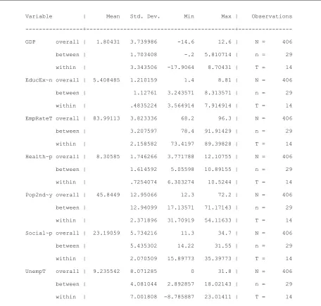
The goal of the summary statistics is to calculate the mean and the standard deviation and break this down for between and within variation. For example, we have the min and max GDP and if we look at between is the average between individuals over time. For within means how much each individual observation differs if you take away the overall mean.

(8)

Licensed under Creative Common Page 35 Figure 1: Summery Statistics from STATA

Variable | Mean Std. Dev. Min Max | Observations

---+---+---

GDP overall | 1.80431 3.739986 -14.6 12.6 | N = 406

between | 1.703408 -.2 5.810714 | n = 29

within | 3.343506 -17.9064 8.70431 | T = 14

EducEx~n overall | 5.408485 1.210159 1.4 8.81 | N = 406

between | 1.12761 3.243571 8.313571 | n = 29

within | .4835224 3.564914 7.914914 | T = 14

EmpRateT overall | 83.99113 3.823336 68.2 96.3 | N = 406

between | 3.207597 78.4 91.91429 | n = 29

within | 2.158582 73.4197 89.39828 | T = 14

Health~p overall | 8.30585 1.746266 3.771788 12.10755 | N = 406

between | 1.614592 5.05598 10.89155 | n = 29

within | .7254074 6.303274 10.5244 | T = 14

Pop2nd~y overall | 45.8449 12.95066 12.3 72.2 | N = 406

between | 12.94099 17.13571 71.17143 | n = 29

within | 2.371896 31.70919 54.11633 | T = 14

Social~p overall | 23.19059 5.734216 11.3 34.7 | N = 406

between | 5.435302 14.22 31.55 | n = 29

within | 2.070509 15.89773 35.39773 | T = 14

UnempT overall | 9.235542 8.071285 0 31.8 | N = 406

between | 4.081044 2.892857 18.02143 | n = 29

within | 7.001808 -8.785887 23.01411 | T = 14

(9)

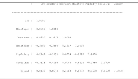
Licensed under Creative Common Page 36 Table 1. Correlation Matrix

| GDP EducEx~n EmpRateT Health~p Pop2nd~y Social~p UnempT

---+---

GDP | 1.0000

EducExpen | -0.0857 1.0000

EmpRateT | 0.0950 0.3313 1.0000

HealthExp | -0.3582 0.3480 0.1217 1.0000

Pop2ndary | 0.2449 -0.1131 0.0334 -0.2526 1.0000

SocialExp | -0.3813 0.4095 0.0046 0.8424 -0.1380 1.0000

UnempT | 0.0139 0.0573 0.1689 -0.0772 -0.1580 -0.0570 1.0000

We test whether the variables are stationary by using Levin-Lin-Chu unit-root test.

Levin-Lin-Chu unit-root test for GDP

---

Ho: Panels contain unit roots Number of panels = 29

Ha: Panels are stationary Number of periods = 14

AR parameter: Common Asymptotics: N/T -> 0

Panel means: Included

Time trend: Included

ADF regressions: 1 lag

LR variance: Bartlett kernel, 7.00 lags average (chosen by LLC)

---

Statistic p-value

---

Unadjusted t -18.0812

(10)

Licensed under Creative Common Page 37 Here we use the LLC test to determine whether the series GDP contains a unit root. The header of the output summarizes the exact specification of the test and dataset. Because we did not specify the no constant option, the test allowed for panel-specific means. On average, p = 1 lag of the dependent variable were included as regressors in the ADF regressions. By default, xt unitroot estimated the long-run variance of the variable by using a Bartlett kernel with an average of 7 lags. The LLC test statistic is significantly less than zero (p < 0.00005), so we reject the null hypothesis of a unit-root in favor of the alternative that the GDP is stationary. We perform the same tests for the other 5 variables and we reject the null hypothesis for all of them meaning that these are stationary as well.

EMPIRICAL RESULTS

The first estimator we use is the pooled OLS estimator. This type of model tells us the relationship between the variables without taking into consideration the countries and the time. The model has the following structure:

𝐺𝐷𝑃𝑖𝑡 = −5.71 + 0.6 ∗ 𝐺𝐷𝑃𝑖𝑡 −1+ 0.108 ∗ 𝐸𝑚𝑝𝑅𝑎𝑡𝑒𝑇𝑖𝑡+ 0.33 ∗ 𝐻𝑒𝑎𝑙𝑡ℎ𝐸𝑥𝑝 𝑖𝑡

+ 0.068 ∗ 𝑃𝑜𝑝2𝑛𝑑𝑎𝑟𝑦 𝑖𝑡− 0.35 ∗ 𝑆𝑜𝑐𝑖𝑎𝑙𝐸𝑥𝑝 𝑖𝑡+ 0.07 ∗ 𝑈𝑛𝑒𝑚𝑝𝑇𝑖𝑡

First of all, the results generally show that higher values of education expenditure are associated with higher values of economic growth. The way we can interpret the results is that an additional point of expenditure with education would lead to 0.108points of economic growth. The economic growth is negatively influenced by social expenditures and positively influenced by the GDP in the previous period. We observe that all the coefficients are significant to explain the economic growth. The Prob>F is 0, which means the model is significant.

Table 2. Model Results using Pooled OLS Estimator Source | SS df MS Number of obs = 377

---+--- F( 6, 370) = 65.89

Model | 2809.42184 6 468.236973 Prob > F = 0.0000

Residual | 2629.50185 370 7.10676176 R-squared = 0.5165

---+--- Adj R-squared = 0.5087

Total | 5438.92369 376 14.4652226 Root MSE = 2.6659

---

GDP | Coef. Std. Err. t P>|t| [95% Conf. Interval]

---+---

(11)

Licensed under Creative Common Page 38 HealthExp | .337853 .1636835 2.06 0.040 .0159865 .6597196

Pop2ndary | .0680089 .0115872 5.87 0.000 .0452238 .090794

SocialExp | -.3526275 .0474609 -7.43 0.000 -.4459544 -.2593006

UnempT | .07182 .0181547 3.96 0.000 .0361207 .1075194

GDP |

D1. | .6015181 .0384654 15.64 0.000 .5258798 .6771564

_cons | -5.719792 3.157014 -1.81 0.071 -11.92773 .4881476

---

The second estimator used is the between estimator and by using this kind of estimator it means that all the data got averaged first. In the between estimator, we compare an individual with the other individuals. If the countries have one more unit of social expenditure, they would have 0.212 less units of growth. There is also a negative relationship between education expenditure and GDP, showing that if the expenses in the previous year are increased with 1%, the GDP will decrease with 5%. If the population with secondary attainment increases with 1%, the GDP will increase 0.039%. The lag of the health expenditure variables not significant to explain the growth. We observe that 𝑅2_{is broken down into between and within variation and}

overall this has a high value of 92%.

Table 3. Model Results using Between Estimator

Between regression (regression on group means) Number of obs = 377

Group variable: statenum Number of groups = 29

R-sq: within = 0.3784 Obs per group: min = 13

between = 0.8992 avg = 13.0

overall = 0.3980 max = 13

F(6,22) = 32.70

sd(u_i + avg(e_i.))= .6365485 Prob > F = 0.0000

---

---+---

GDP |

(12)

Licensed under Creative Common Page 39 EducExpen |

D1. | -5.442884 1.88069 -2.89 0.008 -9.343197 -1.542571

EmpRateT |

D1. | .9661981 .395641 2.44 0.023 .1456889 1.786707

Pop2ndary | .0395875 .0118677 3.34 0.003 .0149753 .0641997

HealthExp |

D1. | 2.15316 1.889167 1.14 0.267 -1.764732 6.071052

SocialExp | -.2121962 .0235697 -9.00 0.000 -.2610769 -.1633156

_cons | 5.303413 .8595387 6.17 0.000 3.520839 7.085987

𝐺𝐷𝑃𝑖𝑡= 5.3 + 1.81𝐺𝐷𝑃𝑖𝑡 −1+ 0.96𝐸𝑚𝑝𝑅𝑎𝑡𝑒𝑇𝑖𝑡− 5.44 𝐸𝑑𝑢𝑐𝐸𝑥𝑝𝑒𝑛𝑖𝑡+ 0.068𝑃𝑜𝑝2𝑛𝑑𝑎𝑟𝑦 𝑖𝑡

− 0.21𝑆𝑜𝑐𝑖𝑎𝑙𝐸𝑥𝑝 𝑖𝑡+ 02.15𝐻𝑒𝑎𝑙𝑡ℎ𝐸𝑥𝑝𝑖𝑡

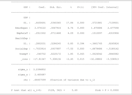
The fixed effects model allows for heterogeneity among the countries but the intercept does not vary over time. From the below results we can see that F statistic is 32.7 and p value is 0, which means that all the coefficients of this model are not equal to 0 and the model is very good and fitted.

For the within estimator below, we compare the employment rate with tertiary with its own average. So, if a country has one more unit of employment rate in comparison to the average, they would have 0.29more units of economic growth. Also, if the GDP per capita of a country at t-1 is higher with 1%, the GDP at t would increase with 0.64 %. If the social expenditures are increased with 1% in comparison to the average, the GDP decreases with 0.7%. All the coefficients are significant except for the health expenditure coefficient in the previous period.

Rho is the percent of the variation explained by individual specific effects and in the below model this has a high value which shows again the significance of the model.

𝐺𝐷𝑃𝑖𝑡 = −17.9 + 0.64𝐺𝐷𝑃𝑖𝑡 −1+ 0.29𝐸𝑚𝑝𝑅𝑎𝑡𝑒𝑇𝑖𝑡+ 2.07 𝐸𝑑𝑢𝑐𝐸𝑥𝑝𝑒𝑛𝑖𝑡+ 0.04𝑈𝑛𝑒𝑚𝑝𝑇 𝑖𝑡

(13)

Licensed under Creative Common Page 40 Table 4. Model Results using Fixed Effects Estimator

---

---+---

GDP |

D1. | .6430691 .0360365 17.84 0.000 .5721881 .7139501

EducExpen | 2.074122 .3067916 6.76 0.000 1.470686 2.677558

EmpRateT | .2911502 .0711468 4.09 0.000 .1512097 .4310906

HealthExp |

D1. | .2802031 .3286245 0.85 0.394 -.3661765 .9265826

SocialExp | -.7033914 .0937897 -7.50 0.000 -.8878686 -.5189142

UnempT | .040702 .0220172 1.85 0.065 -.0026042 .0840082

_cons | -17.91347 7.308136 -2.45 0.015 -32.28802 -3.538913

---+---

sigma_u | 3.2396852

sigma_e | 2.405687

rho | .64457599 (fraction of variance due to u_i)

---

F test that all u_i=0: F(28, 342) = 5.49 Prob > F = 0.0000

The last estimator used is the random effects estimator. This model assumes that the individual-specific effects are distributed independently of the regressors and are included in the error term. If the social expenditures increase with 1% the GDP per capita will decrease with 0.3%. We observe that the p value is less than 0.05, which means the model is significant.

Table 5. Model Results using Random Effects Estimator

Random-effects GLS regression Number of obs = 377

between = 0.7164 avg = 13.0

Wald chi2(6) = 374.80

(14)

Licensed under Creative Common Page 41 ---

GDP | Coef. Std. Err. z P>|z| [95% Conf. Interval]

---+---

GDP |

D1. | .6071821 .037866 16.04 0.000 .5329661 .6813981

EmpRateT | .1308599 .042423 3.08 0.002 .0477123 .2140075

Pop2ndary | .0681618 .0134483 5.07 0.000 .0418036 .0945201

HealthExp | .3946644 .1798098 2.19 0.028 .0422436 .7470852

SocialExp | -.3779356 .0529037 -7.14 0.000 -.4816249 -.2742462

UnempT | .0733652 .0185732 3.95 0.000 .0369623 .1097681

_cons | -7.491951 3.551275 -2.11 0.035 -14.45232 -.5315789

---+---

sigma_u | .47700221

sigma_e | 2.5181024

---

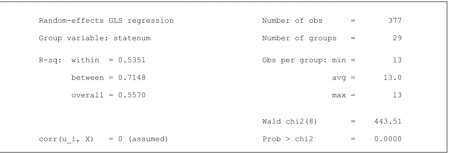
Based on the cluster analysis performed, we introduce a dummy variable to classify the countries into developed and developing countries. This takes the value 1 if the country is developed and 0 if it is a developing country. Next we estimate the random effects model with the dummy variable and the results are the following.

The p value shows that the model is significant but again the coefficient of unemployment shows that this cannot explain the GDP. The coefficient of the dummy variable is 0.77, which means that if the country is a developed one, the GDP per capita grows, on average, with 0.77% points.

Table 7. Model Results using Random Effects Estimator with a dummy variable

Random-effects GLS regression Number of obs = 377

between = 0.7148 avg = 13.0

Wald chi2(8) = 443.51

(15)

Licensed under Creative Common Page 42 ---

GDP | Coef. Std. Err. z P>|z| [95% Conf. Interval]

---+---

GDP |

D1. | .6768793 .0376238 17.99 0.000 .603138 .7506205

|

EducExpen | .2549894 .1576323 1.62 0.106 -.0539642 .5639429

EmpRateT | .1637634 .0433598 3.78 0.000 .0787798 .2487469

Pop2ndary | .0612279 .0140513 4.36 0.000 .033688 .0887679

HealthExp | .342122 .1779678 1.92 0.055 -.0066884 .6909324

SocialExp | -.4071578 .0579224 -7.03 0.000 -.5206837 -.2936319

|

UnempT |

D1. | .1928087 .0276084 6.98 0.000 .1386972 .2469201

|

Bin | .7787879 .457287 1.70 0.089 -.1174781 1.675054

_cons | -9.524912 3.600736 -2.65 0.008 -16.58223 -2.467599

---+---

sigma_u | .5571429

sigma_e | 2.2966375

---

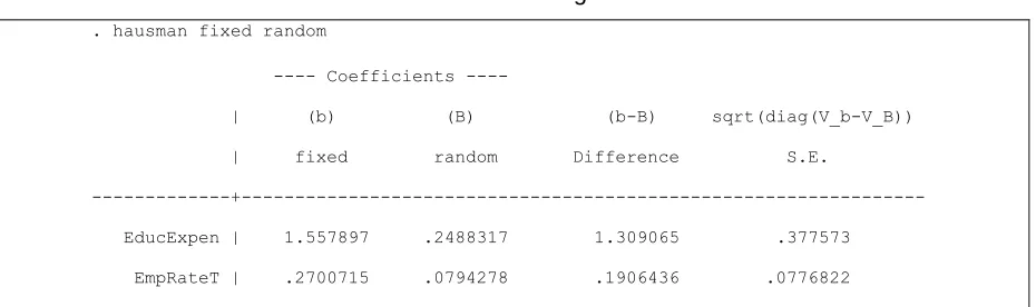
We perform two tests in order to choose from the above estimated models: Hausman test for fixed versus random effects model and BrEuropesch-Pagan LM test for random effects versus OLS.

Table 9. Breusc-Pagan LM test . hausman fixed random

---- Coefficients ----

| (b) (B) (b-B) sqrt(diag(V_b-V_B))

| fixed random Difference S.E.

---+---

EducExpen | 1.557897 .2488317 1.309065 .377573

(16)

Licensed under Creative Common Page 43 HealthExp | -.7489016 -.1488296 -.600072 .2366258

Pop2ndary | .0133818 .0563978 -.043016 .0714233

SocialExp | -.2393197 -.223039 -.0162807 .1201198

UnempT | -.0106221 .0004925 -.0111147 .0196538

---

b = consistent under Ho and Ha; obtained from xtreg

B = inconsistent under Ha, efficient under Ho; obtained from xtreg

Test: Ho: difference in coefficients not systematic

chi2(6) = (b-B)'[(V_b-V_B)^(-1)](b-B)

= 20.83

Prob>chi2 = 0.0020

Breusch and Pagan Lagrangian multiplier test for random effects

GDP[statenum,t] = Xb + u[statenum] + e[statenum,t]

Estimated results:

| Var sd = sqrt(Var)

---+---

GDP | 13.98749 3.739986

e | 10.9312 3.306236

u | .1129745 .3361168

Test: Var(u) = 0

chibar2(01) = 0.02

Prob > chibar2 = 0.4494

The results show that we have significant results and we shouldn‟t be using the pooled OLS

(17)

Licensed under Creative Common Page 44

CONCLUSIONS

Studies on the relationship between human capital and economic growth for the case of Europe countries, using panel data models are not very common because of the availability of data. We used a panel data model on a set of 29 European countries observed during 2000 and 2013 to capture the effects in time and space of six macroeconomic variables on economic growth. More specifically, we have used a pooled OLS, a fixed, random and dynamic panel data models these to detect both direct and indirect effects of human capital indicators on economic growth.

Preliminary results from pooled OLS analysis show that employment rate, health expenditure and population with secondary attainment have a positive impact on growth. Fixed effects panel data estimates suggest that one percent increase in education, proxied by education expenditure will lead to 2% increase in the GDP. The results confirm the positive link found in the literature.

The obtained results show a positive correlation between education expenditure employment rate by tertiary education, health expenditure, population with secondary education attainment and economic growth. All the estimators show there is negative relationship between social protection expenditure and GDP per capita.

For future research it will be interesting to add the Human Development Indicator as a dependent variable and a proxy for economic development. Furthermore, the purpose will be to include in the research groups of developed and developing countries in order to see if there is a difference between the impact of human resources indicators on the economic development in emerging and developed economies.

REFERENCES

Afonso, A., & Alegre, J. G. (2011). Economic growth and budgetary components: A panel assessment for the EU. Empirical Economics, 41, 703–723. http://doi.org/10.1007/s00181-010-0400-9

Apergis, N., Filippidis, I., & Economidou, C. (2007). Financial deepening and economic growth linkages: A panel data analysis. Review of World Economics, 143(1994), 179–198. http://doi.org/10.1007/s10290-007-0102-3

Barguellil, A., Zaiem, M. H., & Zmami, M. (2013). Remittances , Education and Economic Growth A Panel Data Analysis. Journal of Business Studies Quarterly, 4(3), 1–11.

Barro, R. J. (2006). Education and economic growth., 2, 277–304.

Barros, C. P., & Alves, F. M. P. (2003). Human Capital and Economic Growth Revisited: A Dynamic Panel Data Study. International Advances in Economic Research, 9, 218–226. http://doi.org/10.1007/BF02295445

Bensi, M. T., Black, D. C., & Dowd, M. R. (2004). The education/growth relationship: Evidence from real state panel data. Contemporary Economic Policy, 22, 281–298. http://doi.org/10.1093/cep/byh020

(18)

Licensed under Creative Common Page 45 Fernald, J. G., & Jones, C. I. (2014). The future of US economic growth. American Economic Review, 104(5), 44–49. http://doi.org/10.1257/aer.104.5.44

Jaunky, V. C. (2012). Democracy and economic growth in Sub-Saharan Africa: a panel data approach. Empirical Economics, 869, 987–1008. http://doi.org/10.1007/s00181-012-0633-x

Jin, L., & Jin, J. C. (2014). Internet Education and Economic Growth: Evidence from Cross-Country Regressions, 78–94. http://doi.org/10.3390/economies2010078

Kumar, C. S. (2006). Human Capital and Growth Empirics. The Journal of Developing Areas, 40, 153– 179. http://doi.org/10.1353/jda.2007.0006

Magoutas, A. I., Papadogonas, T. a, & Sfakianakis, G. (2012). Market Structure, Education and growth. International Journal of Business & Social Science, 3(12), 88–95.

Mahmood, T., & Ahmad, E. (2014). Output growth and investment dynamics in Finland : a panel data analysis, 777–801. http://doi.org/10.1007/s10663-013-9236-9

McDonald, S., & Roberts, J. (2002). Growth and multiple forms of human capital in an augmented Solow model: A panel data investigation. Economics Letters, 74, 271–276. http://doi.org/10.1016/S0165-1765(01)00539-0

Mends-Brew, E., Avordeh, T. K., & Forson-Yeboah, D. (2012). Modelling Economic Growth in Ghana. European Scientific Journal, 8(12).

Reza, F., & Widodo, T. (2013). The Impact Of Education On Economic Growth. Journal of Indonesian Economy and Business, 28(1), 23–44.

Seetanah, B. (2009). the Economic Importance of Education : Evidence From Africa Using Dynamic Panel Data Analysis, XII(1), 137–157.

Sequeira, T. N., & Martins, E. V. (2008). Education public financing and economic growth: An endogenous growth model versus evidence. Empirical Economics, 35, 361–377. http://doi.org/10.1007/s00181-007-0162-1

Tatoglu, F. Y. (2011). The Relationship between Human Capital Investment and Economic Growth: A Panel Error Correction Model. Journal of Economic and Social Research, 13(1), 75–88.

Ulah, Farid; Rauf, A. (2013). IMPACTS OF MACROECONOMIC VARIABLES ON ECONOMIC GROWTH : A PANEL DATA ANALYSIS OF SELECTED ASIAN COUNTRIES. International Journal of Information, Business and Management, 5(2), 4–13.

Yardimcio, Fatih; Gurdal, Temel;‟ Altundemir, M. (2014). Education and Economic Growth : A Panel Cointegration Approach in OECD Countries ( 1980-2008 ). Education and Science, 39(173), 1–12.