Evaluating Deep Learning Paradigms With TensorFlow And Keras For Software Effort Estimation

2753

Evaluating Deep Learning Paradigms with

TensorFlow and Keras for Software Effort

Estimation

Sreekumar P. Pillai, Dr.T.Radha Ramanan, Dr.S.D.Madhu Kumar

Abstract— Deep learning is an arm of Artificial Intelligence that uses deep neural networks to achieve artificial intelligence. It has made its mark in computer vision, speech recognition, language processing, and automatic engines. Google made a significant contribution to AI technologies by releasing TensorFlow (TF), its proprietary AI platform, in 2015, as an open-source software library to define, train and deploy learning models, including Machine Learning and Deep Learning. In this study, we aim to improve software estimation using the most recent deep learning paradigms. We employ TensorFlow and a high-level wrapper API to TF and evaluate a composite hyper-parameter tuning method employing the Cartesian grid and random search. We observe significant performance improvement, achieved (29.8%) from the base model, using the hybrid hyper-parameter tuning methodology. However, even While literature reports significant performance in cognitive imaging with TF and Keras, we have not been able to validate any substantial improvement in prediction, in the case of a software effort estimation data such as ISBSG 2018 by employing these techniques. Index Terms— Software Effort Estimation, Software Cost Estimation, Effort Prediction, Feature Engineering, Artificial intelligence, Neural Networks, Deep Learning, Machine Learning, TensorFlow, Keras, Hyperparameters.

——————————  ——————————

1 I

MODERN algorithms further the growth of scientific and technological advancements in computing intelligence. This is reflected in computer vision systems, natural language processing, speech synthesis, weather predictions and autonomous vehicles. Machine Learning and Deep Learning form the crux of AI. Deep Learning is a group of algorithms that uses complex layers of neural networks that can manage very complex functions with data of any distribution. This can be used to solve, classification, regression, or any other kind of unsupervised tasks such as automated vision. Deep Learning came into the forefront in the last few years due to the lower cost of data retention mechanisms facilitating the availability of huge amounts of data for computational analysis. Additionally, the massive parallel processing power provided by Graphical Processing Units (GPUs) have nurtured the growth of Deep Learning. New hardware, new algorithms, and functions have tremendously helped the cause of deep learning. Many different software platforms have been designed to employ these mathematical algorithms to solve practical problems. There is commercial and community-based software like H2o, TensorFlow, and Keras. Google added its proprietary ML platform as an open-source tool in November 2015 [1]. TensorFlow provides low-level control over the design of deep neural networks using a new paradigm called computational graphs. While this is complex for everyone to use, Keras provides a higher-level API to interact with TensorFlow core. Keras also has the GPU version to interact with the GPU powered TensorFlow back-end. TensorBoard, a web application shipped along with TensorFlow, helps interactively visualize the computational graph. Python was the de-facto language used to interface with TF. Recently, Keras has released their version of APIs for the R statistical programming language. All this software enables parallel and distributed processing of data in heterogeneous systems and can represent the many activations, transformation, and regularization functions with thousands of libraries in R and python. Despite the heavy influx of ML algorithms, the tuning of their hyperparameters still remains a gruesome task, and proper tuning is required to get the best performance out of any model [2]. Automatic feature selection is a norm especially in Convolutional Neural Networks (CNNs) applied in imaging and speech synthesis. Many scholars attempted feature

2754

Figure 1:Architecture of the Base Neural Network

2

P

S

Estimation is a critical business function in all domains. In the domain of Software Engineering, this takes on additional importance and complexity due to the intangible nature of the work product. Mathematically, estimation becomes a prediction problem, and with the low accuracy from the existing models, scholars and industry specialists are engaged in a continuous attempt to improve the efficiency of the existing methodologies. Additionally, in software engineering, it is pertinent to make optimum use of techniques to improve prediction with the limited data available. ML techniques offer a new dimension to software estimation prediction by exploiting the many hidden patterns no not obvious to the naked eye. Our current study is to explore the possibilities in this direction using the ISBSG dataset R1 that has been optimized through feature engineering. ML techniques require an extreme level of tuning of their hyper-parameters. Our experiment aims to identify the best possible neural architecture using TensorFlow and Keras to gain the best accuracy using a hybrid hyper-parameter selection method.

Figure 2:The Experiment Hardware Environment

3

B

W

In parallel to the growth of Machine Learning, scholars have begun to focus on Feature engineering as distinct from feature

selection, which is already established as a technique in Machine Learning solutions.

3.1 Artificial Neural Network

In the software effort estimation domain, Nassif [7] has experimented with NN. He analyzed four different NN models: Multilayer Perceptron (MLP), General Regression Neural Network (GRNN), Radial Basis Function Neural Network (RBNN), and Cascade Correlation Neural Network (CCNN) with each other on standard accuracy metrics. His finding was that all the four models tend to overfit in 80% of the datasets.

3.2 Feature Engineering

Feature engineering constructs suitable features from the existing ones leading to the increased predictive performance of the ML model and transforms the current data using arithmetic and aggregate operators. Transformation of the data helps scale a specific feature or convert a non-linear relation between a feature and a target class into a linear association, to make it easier to be consumed by the ML algorithm. Feature engineering involves creating new features from the existing ones to improve the performance of an algorithmic model, at the source. Kang.et.al [8], in their book on Feature-Oriented Domain Analysis‖ states that features should capture the user‘s understanding of capabilities of the application domain. Brazdil, Pavel discusses many induction-based techniques in his paper‖ Constructive Induction of Continuous Spaces‖ [9]. Turner.et.al [10] was the first one to coin the term ‘Feature Engineering‖ in their seminal paper on the topic in 1999, and they set out‖ promotion of features as first-class objects within the software process‖ as the goal for feature engineering. Liu.et.al summarizes many discretization techniques to achieve improved accuracy as a feature engineering technique for continuous values [11]. Feature Engineering techniques in knowledge-based construction was elaborated by Re.et.al [12] and further employed in question-answer selection solution by Aliaksei Severyn [13] evidencing an efficiency improvement of 22%. We use feature engineering techniques to improve data retention in the base ISBSG dataset as covered in a previous experiment [14].

4

T

F

K

TensorFlow is Google‘s framework for machine learning. Each new version of the platform brings a wide range of capabilities and features. TensorFlow has a steep learning curve; but once employed, highly sophisticated machine-learning applications can be designed and executed at high-performance levels.

4.1 TensorFlow Architecture

TensorFlow envisages a data flow graph language to express the computations done by the algorithms. These graphs can be assigned to local as well as distributed hardware improving the efficiency of the software and the hardware.

2755 Tensors: In TensorFlow, tensors are symbolic handles that

represent the output of a computing operation. During operations, a tensor object is passed connecting the input and output carrying data through the TensorFlow graph.

4.2 TensorFlow Data Types:

TensorFlow applications can be written in several different languages, such as Python, C++, and Java. No matter which language is used, the data types remain common that are specific to TensorFlow.

Tensors and placeholders: Tensors are instances of the Tensor class, and it serves like a general-purpose multi-dimensional array. A placeholder is also a Tensor, but instead of being initialized in code, it receives data from a session that will be valid during one execution of the session. Placeholders make it possible to update a tensor‘s content from one session execution to the next.

Graphs: A graph is a container like a list or a tuple. Only one graph can be active at a time, and when you code an operation that accepts tensors or variables, the tensors, variables, and operation are stored as elements in the graph. When you create an optimizer and call its minimize method, TensorFlow stores the resulting operation in the graph.

Sessions: A session is an environment within which operations are performed. The session helps manage the required computing resources. The TensorFlow computational graph exists within the session. Graphs store operations and perform computations within the environment. One of the responsibilities of a session is to encapsulate the allocation and management of resources such as variable buffers [8].

Optimizer: The objective of machine learning is to represent a real-world scenario as closely as possible. It starts at an arbitrary point and progressively refines the models to achieve the optimum state. Optimizer algorithms are different mechanisms defined to achieve this. TensorFlow supports most of these algorithms within its default framework.

Variables: Variables hold data and get modified as part of the computing operation and the optimization process. Derived values as well as original data are stored as variables in TensorFlow.

Estimators: The estimator class in TensorFlow provides a higher-level API to avoid the user needing to deal with sessions and graphs, which are low-level structures. An estimator encapsulates an algorithm that is used for learning. All estimators define the train, evaluate, and predict methods. TensorFlow also provides an interactive visualization to help non-expert users get an intuitive understanding of the neural network that is being experimented, called the TensorFlow Playground. Users can experiment with their neural network architecture and see the output by manipulating the values in a visual manner rather than coding.

4.3 Keras

Keras is a high-level API written in Python and R that forms a user-friendly wrapper for the TensorFlow, CNTK, or Theano deep learning libraries. Keras can execute on CPU or GPU hardware employing hundreds of parallel threads, speeding up

the machine learning processing. Keras envisages a model as a sequence of configurable modules that can be plugged together seamlessly. Neural network layers, cost functions, optimizers, regularization schemes, and activation functions are all constructed as modules that can be combined to create flexible NN models.

5

N

N

A

Our neural network diagram is shown in the Fig.1. The architecture of the neural network plays a vital part in the performance of the learning machine.

5.1 A wide or deep network topology?

There is no hard and fast principle when it comes to the neural net topology. A single wide neural networ k will be able to learn any function given enough training data. However, using extremely shallow networks force the machine to memorize the training data reducing its generalizing capability. These kinds of models work poorly when fed with new data Smith, Leslie N [16]. Multiple layers can learn the features and their relationships at different levels of abstraction. Multi-Layered neural network topology will generalize the training data in a much better way providing better accuracy. Using a deep and wide topology also inherits the disadvantages of the wide network resulting in poor generalization capability. There is more or memorization happening with the additional burden of a huge network that will over-fit the training data and taking longer to train. Deep networks need more computing to be trained. So, a deep Vs. Wide optimum trade-off is recommended. Our network architecture comprises of input layer, hidden layers and an output layer. All our layers are dense, all nodes are connected to other nodes in the subsequent layer. This is a multi-layer perceptron model with back propagation. The Keras API implements back propagation automatically. The network architecture is shown in Fig. 1. We employ RELU, Linear, and Exponential for the regression based on previous studies. We choose Adam optimization for the optimization algorithm since it is well represented in literature. Adam is Adaptive moment estimation (Adam = RMSprop + Momentum). It has relatively low memory requirements (though higher than gradient descent and gradient descent with momentum) Usually works well even with little tuning of hyperparameters [17]. In our regression problem, we use MSE for our loss function. The objective is to identify the architecture with the least Mean Squared Error. The is the most used [18] loss function for regression. MSE is derived by taking the mean of the sum of the square of the distances between actual and predicted values.

The equation for MSE is as given in Eq. 1.

∑ ( ̂)

(1)

5.2 Hardware and Software Configuration

2756

6

M

We employed a Feature Engineered dataset from one of our previous experiments in this experiment too. The data that we used in this study is from ISBSG (Release 1, 2018, February). This dataset contains information on 8261 projects executed globally and collected from volunteering organizations. The projects were submitted from 26 countries [19].

6.1 Feature Selection

We selected the eight critical variables from the ISBSG 2018 R1 dataset that represents the software effort estimation problem based on the literature and our experiments on the subject [20], [21]. A brief description of these variables and their relevance to the experiment is detailed in the following sub-sections.

Functional Size

The un-adjusted Functional size is the raw size of the developed software without accounting for any complexity of the environment in which it is developed. [22].

Value Adjustment Factor

The VAF is a multiplication factor derived based on 14 environmental characteristics of software project. VAF can be anywhere from 0.65 to 1.35 and modifies the software size to reflect impacts due to the environmental factors.

Development Type

The type of software developed can be a completely new one based on user requirement, a redevelopment of existing applications or minor enhancements to them. This is captured as the Development Type variable. Software productivity varies based on the type of development work [23] and this will be reflected in the effort.

Language Type

New generation programming languages offer significant productivity since they are more evolved. The lang.type

variable captures the generation of the language employed in the development.

Mean Product Delivery Rate

Product Delivery Rate refers to the effort required to deliver software product of unit size. We feature engineered the previous year‘s mean product delivery rate as part of the dataset from a previous feature experiment we conducted [14].

Team Size Group

The average number of people employed in the team impacts the project effort. A large team brings communication overhead and other dysfunctions [24]. Team size and the language type has been analyzed in detail by Jiang and Comstock [25] evidencing their significance.

Industry Sector

The complexity of a piece of software is tied to the nature of the industry that uses it. Software developed for defense and the health-care industry falls into the category of highly complex ones as against the ones in the Education domain. Software productivity also varies across industry domains along with complexity [26]. To enhance accuracy of parametric models, scholars have proposed grouping of projects based on productivity [27],[28].

Work Summary Effort (Dependent Variable)

The summ. weffort represents the overall effort required to develop a piece of software and forms the independent variable. 90% of software development cost is from the human effort involved; estimating this is the objective of any software effort estimation study.

6.2 Data Pre-processing

During the data pre-processing, we selected only rows that had passed the quality standards based on the rating set by ISBSG as A or B. Only those projects have been included where the data has been directly recorded and the sizing measure is Function Point.

6.3 Outliers

To eliminate outliers, we used a multivariate outlier detection procedure using Cook‘s distance [29], [30]. Outliers are detected based on influences from all numerical variables together. Yeong et al. [31] mention a procedure for outlier detection using multivariate analysis, further elaborated by Kannan and Manoj[32]. The influence of each data point (row) in the dataset is computed based on the equation:

6.4 Normalization

We normalized both the original as well as the engineered dataset using BoxCox transformation function, which gave the best outcome compared with the other options we tried employing lognormal and cube-root transformations.

∑ ( ̂ ̂ ( ))

(2)

6.5 Modeling & Testing

We used the train and test sets to build and test our linear regression model by splitting the dataset using the 80:20 ratio. We built the model using the training set reserving the test set to validate the model accuracy with independent data.

In all our simulations we calculated the mean squared error (MSE) with a batch size of 32. We compare the four following We compare the following models adam optimiser, relu, softmax, learning rate:

TensorFlow — Single Layer Perceptron Usage of initializers Initializations configure the way to set the initial random weights of Keras layers.

6.6 Scaling of data

Quite different from Z-score normalization and median and MAD method, the min-max method retains the original distribution of the variables. We use min-max normalization to scale the data. The initial network diagram with the nodes and weights are show in the Fig. 1. Figure 3 visualizes the computed neural network. Our base model has 2, and 4 neurons in its hidden layer. The black lines show the connections with weights. The weights are calculated using the back-propagation algorithm explained earlier. The blue line is the displays the bias term.

6.7 Model Accuracy

2757 (MRE) measures the relative error of the estimate and is

defined as [28]

The Mean Magnitude of Relative Error (MMRE) is expressed as:

∑

| |

(4)

Prediction (PRED) is determined for n projects; the prediction at level P is defined as:

( ) (5)

K is the number of projects where the MRE is less than or equals p. Desirable MMRE and PRED thresholds were first published by [34], and subsequently by other scholars [35].

6.8 Feature Engineering

We performed the following feature engineering techniques on the original data as part of the experiment.

Missing Value Imputation

Standard imputation has been performed on ISBSG dataset by Sentas and Angelis [23], Shepperd and Cartwright [36],[37], Song et al. [38], Sehra et al. [39], and recently by Mittas et al.[40]. We performed imputation of missing values using Buuren‘s, ‗Multivariate Imputation‘ method [41] as implemented in the mice‘ R‘ package. Within the ISBSG dataset version we used, specific projects have captured the unadjusted Function Points, and others measured Adjusted FP along with VAF. We removed rows only where both these values are non-existent. In cases where two of these values are present, we have derived the missing values based on equation (1). This helps us retain close to 30% of the rows missing VAF in the original dataset. Data imputation is done for Language Type (lang.type) and Team Size Group(team.size.gp) variables based on multivariate imputation further evidenced in the papers by Cartwright[37], and recently by Lee [42]. The feature engineering experiment was conducted in the following order to arrive at the optimum set of features.

New Transformed Features

Software Product Delivery Rate (PDR) is a metric used by ISBSG to denote the productivity of software Development based on each product. This is a derived measure from the quantity of software produced and the time taken to produce it. This is a lag measure since this is available only once the project is complete. We hypothesize that the historical productivity of a team is indicative of the future effort required by any team. The software productivity rate is also dependent on the Industry sector (complexity of software varies based on the nature of the domain), the programming language generation, and the skill availability in the team. To account for these variations in the software production rate, we engineered a feature that combined all four elements. Our engineered productivity average referred to the mean of the productivity figures for the preceding year grouped against all

these dependent categorical features. Due to this transformation, we have lost information for the year 1989, the

first year in the dataset since there is no previous year data to substitute. Taking the mean of software production rate against all these features also means that there should be adequate records matching all the combinations of these features. Since this is not the case with the ISBSG dataset, we accept this loss of information bringing down the number of records to 3035.

Capturing Missing values

We wanted to capture‖ missingness‖ of the features to ascertain their representational value to the prediction capability of our model. We created an ―is.Na‖ column for the categorical variables in the dataset.

Imputation for Missing Values

We imputed the original ind.sector feature with values from the same column using CART. The CART algorithm is based on Classification and Regression Trees by Breiman et al. [43]. A CART is a binary decision tree constructed through splitting each node of a tree, recursively starting with the base node. The ‘R‘ package MICE implements CART [41] for imputation.

Imputing Value Adjustment Factor

In the original dataset, fields are missing for this column. We imputed the missing values in this column using the formula:

(6)

Where, AFP = Adjusted FP, UAFP = Unadjusted Function Point. Wherever this value could not be derived, we substituted the value with 1. This substitution implies that no external factors influencing the software development effort and the factor representing the general system characteristics equate to 1.

Segmentation based on Homogeneous Labels

Segmentation has improved the accuracy of effort estimates [44], and [45]. Additionally, fewer number of variables increases the model‘s manageability. We conducted the ANOVA test for categorical variables and found the presence of homogenous groups. We employed the multiple comparison procedure proposed by Donoghue [46] to visualize the homogeneous groups and further implemented in the ‗R‘ package ―MultCompView,‖ by Graves et al. [47].

Development Type - dev.type

The one-way ANOVA test shows a statistically significant difference between the groups (F (2.4038) = 103.7, p = 2e-16). Post-Hoc testing using the Bonferroni adjusted P-value method suggested identical mean values for Re-Development and New Development projects. We combined these two levels into a single value called Development.

Language Type - lang.type

The one-way ANOVA test displays a statistically significant difference between the different groups of the lang.type

| |

2758 variable (F (3.4037) = 5.526, p = 0.000876). Post-Hoc testing

using the Bonferroni adjusted P-value method suggested identical mean effort values for 2GL and ApG languages. We combined these two levels into a single value called ApG.

Industry Sector - ind.sector

One-way ANOVA test done on the ind.sector variable shows statistically significant difference between its groups (F (13.4027) = 19.42, p = 2e-16). Figure 7 shows the homogeneously different groups within this variable based on the test.

The Post-Hoc tests using the Bonferroni adjusted P-value method suggested grouping homogeneous industry sectors to simplify the model and reduce errors. We grouped the categorical variables as in Table 3 based on the ANOVA results.

Columns Dropped after PCA

The team.size.gp and max.team.size are two variables that represent the size of the team employed in the software development process. Doing PCA, we dropped the

max.team.size variable as it was redundant substantiated by its high correlation with the team.size.gp variable. We decided to retain the team.size.gp variable, which provides more insight and is also intuitive to the researcher and practitioner alike. None of the other variables display high collinearity. We also dropped all variables that captured the missing information, and label counts except for Industry Sector (ind.sector) and Development Type (dev.type) that showed representational value. The variables that were employed for the final experiment are indicated in Table 1.

Exploratory Statistics of the Engineered Dataset

The descriptive statistics of the engineered dataset in Table 2. We transformed the variables using the BoxCox transformer implemented in the R package MASS, that has been able to rectify the skew in the data to an acceptable level.

7.EXPERIMENT

Our experiment comprised of three distinct stages: defining the base model, tuning the hyper-parameters and evaluating the results.

7.1 Base Model Definition:

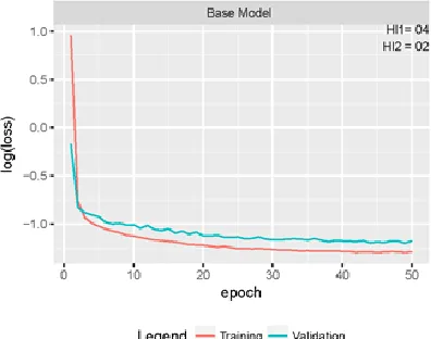
Figure 3:Base Model Scoring History

We created a base model as the starting point, the topology of which is illustrated in Fig.1. This has one input layer, two hidden layers, and one output layer. There are 13 input neurons that represent the predictor variables. The two hidden layers are of 4 and 2 neurons, each based on literature guideline for better generalization[48], and one output neuron representing the response variable. The batch size initially adopted is 4, and the network employ Adam optimizer which is a much acclaimed algorithm for first-order gradient based optimization [17]. Initially, we tested the performance of model for 50 epochs and and recorded the results. The loss values from training and validation is shown in Fig. 3. As observed, the validation error is higher than the training error and there is no convergence.

7.2 Hyper-parameter Tuning:

Hyper-parameter optimization of neural networks is challenging due to their large count. Grid search and random search are two popular methods employed by experimenters. We use a twin step procedure to tune the hyper-parameters. In step 1, we narrow the values of a parameter to a probable range through grid search. In the subsequent one, we identify the best possible value within this limited range through random search.

(Step 1) Optimum Neurons in the Hidden Layers:

The neurons in the hidden layers has an impact on the model performance. To choose the right numbers, we created 60 models with randomly chosen values for each of the hidden layers. MMRE values for each model (combination of neurons) was recorded and plotted as a three dimensional scatter plot as in Fig. 4. The optimum combination is available with a single neuron in the first layer and 7 neurons in the second.

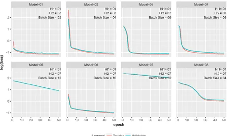
(Step 2) Finding the Best Batch Size:

The batch size determines how many examples are evaluated before updating a weight. Lower sizes create noise as against the higher sizes that take longer time to compute the gradients and impacts the model convergence. Li et al. observes that convergence degrades with increasing batch sizes [49]. In this step, we create 8 different models with batch sizes [2,4,6,8,12,16,32,64] and compare their performances to decide the ideal batch size for the dataset we use. The training and validation plot from the batch size models evidence the optimum batch size is 8 (Model-04) as in Fig. 5, which is used for the next set of optimization.

Table 1:Best Hyper-parameters

No. Model _Model Base _Model Final

1 Batch.Size 4 8

2 Hidden Layer 1 4 1

3 Hidden Layer2 2 7

4 Regu.rate 0.0054

5 LRate 0.0059

6 Epochs 50 100

7 Optimizer Adam Adam

8 Activation Function Relu Relu

9 Loss Function Mae Mae

2759 Recommended learning rates for neural networks range from

0.1 to 1e-06. The best learning rate is anywhere between this range. Practically, it is impossible to test models with values in this entire spectrum. By convention, scholars vary the learning rate by a power of ten. This helps them select the best

learning rate, randomly from a grid of these values. To shorten the scope of this extensive range, we employ a two-step process: in the first step, we identify the best grid within which the learning rate falls.

Figure 4:Base Model Scoring History

We observed that the optimum learning rate lie between the bounds of Model03 and Model04 represented by values 0.01 and 0.001 respectively. In the final step, we randomly choose a value between these two.

(Step 4) Regularization

The two commonly adopted means to reduce over-fitting of datasets are dropouts [50] and regularization. Regularizers allow applying penalties to the layer weights during optimization. These penalties get included into the loss function optimized by the network. We employ L2 regularization to reduce over-fitting and improve the model performance. Regularization rates typically takes values from 0.1 to 1e-06. To narrow down on the accurate regularization rate, we follow a two-step procedure as with the learning rates. The best range of values is identified, and models are created with random values within this range. We obtain the best regularization rate in the range 0.01 to 0.001.

(Step 5) Final Model

The train and validation plot for the final model is shown in Fig. 6. In this step, we built 10 models based on random values for the learning, and regularization rates between the range of values identified in the first stage. The models were created for the optimum batch size of 8 and experiment conducted for 100 epochs with stratified samples over 10 iterations. Table 2 shows the optimum values for the hyper-parameters:

8

R

D

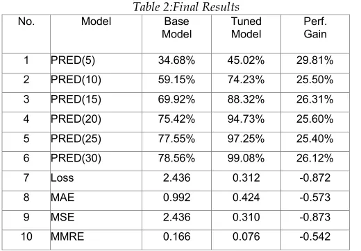
Our results evidence that Tensor Flow and Keras can provide comparable performance in Software effort estimation to that of other models. The model can predict effort with 45% accuracy with a confidence interval of 95%, and with 94.7% accuracy at PRED (20). The results are reported in Table 3. Through a hybrid approach we employed to tune the hyper-parameters, we achieved a performance improvement of 29.81% at the 95% confidence interval.

2760

Table 2:Final Results

No. Model Base

Model

Tuned Model

Perf. Gain

1 PRED(5) 34.68% 45.02% 29.81%

2 PRED(10) 59.15% 74.23% 25.50% 3 PRED(15) 69.92% 88.32% 26.31% 4 PRED(20) 75.42% 94.73% 25.60% 5 PRED(25) 77.55% 97.25% 25.40% 6 PRED(30) 78.56% 99.08% 26.12%

7 Loss 2.436 0.312 -0.872

8 MAE 0.992 0.424 -0.573

9 MSE 2.436 0.310 -0.873

10 MMRE 0.166 0.076 -0.542

MSE=Mean Squared Error, MAE=Mean Absolute Error, MMRE=Mean Magnitude of Relative Error

9LIMITATIONS

This study is based on the publicly available dataset and does not consider the environmental or organizational aspects of software development in terms of development skills or process maturity. While the model encapsulates the global nature of the current day software development process, individual models catering to the specific development organizations might evidence to produce more accurate estimates. ISBSG has limitations to provide a countrywide classification of productivity due to confidentiality agreements which pose a limitation to ascertain whether national productivity impacts the estimated effort, thereby the cost of software development, geographically.

10

C

We evidence that the power of computation graph-based models is in solving complex data in highly multi-dimensional space especially in the unsupervised space with hundreds of features and millions of rows. Employing these in Software Engineering Estimation is an overkill with no significant advantage in terms of accuracy. The hybrid hyper-parameter tuning approach we employed using Cartesian grid with random search evidences excellent tuning capability with high savings in neural network tuning. The research also evidences the use of past productivity in the estimation of future projects and substantiates the intuitive and logical hypothesis that historical productivity can be relied on to estimate future development effort. Additionally, the results of our research will build confidence in software organizations to maintain and use local productivity metrics for future estimation purpose. As the next step, we propose further research using these engineered features to further the research in Software Effort Estimation domain using Deep Learning techniques.

R

[1] M. Abadi, A. Agarwal, E. B. Paul Barham, A. D. Zhifeng Chen, Craig Citro, Greg S. Corrado, I. G. Jeffrey Dean, Matthieu Devin, Sanjay Ghemawat, Y. J. Andrew Harp, Geoffrey Irving, Michael Isard, Rafal Jozefowicz, M. S. Lukasz Kaiser, Manjunath Kudlur, Josh Levenberg, Dan Man´e, J. S. Rajat Monga, Sherry Moore, Derek Murray, Chris Olah, P. T. Benoit Steiner, Ilya Sutskever, Kunal Talwar, F. V. Vincent Vanhoucke, Vijay Vasudevan, M. W. Oriol Vinyals, Pete Warden, Martin Wattenberg, Yuan Yu, X. Zheng.,

TensorFlow: Large-scale machine learning on heterogeneous systems, Methods in Enzymology 101 (1983) 582–598. doi:10.1016/0076-6879(83)01039-3. arXiv:1605.08695.

[2] T. Menzies, M. Shepperd, Special issue on repeatable results in software engineering prediction, Empirical Software Engineering 17 (2012) 1–17. URL: https://doi.org/10.1007/s10664-011-9193-5. doi:10.1007/s10664-011-https://doi.org/10.1007/s10664-011-9193-5.

[3] S. R. Young, D. C. Rose, T. P. Karnowski, S.-H. Lim, R. M. Patton, Optimizing deep learning hyper-parameters through an evolutionary algorithm, in: Proceedings of the Workshop on Machine Learning in High-Performance Computing Environments, November, ACM Digital Library, 2015, pp. 1–5. doi:10.1145/2834892.2834896. [4] L. Song, L. L. Minku, X. Yao, The impact of parameter tuning on

software effort estimation using learning machines, Proceedings of the 9th International Conference on Predictive Models in Software

Engineering - PROMISE ‘13 (2013) 1–10.

doi:10.1145/2499393.2499394.

[5] R. Jeffery, M. Ruhe, I. Wieczorek, Using public domain metrics to estimate software development effort, Proceedings - 7th International Software Metrics Symposium, 2001 (2001) 16 –27. doi:10.1109/METRIC.2001.915512.

[6] G. D. Boetticher, Using Machine Learning to Predict Project Effort: Empirical Case Studies in Data-Starved Domains, Model Based Requirements Workshop (2001) 17–24. doi:10.1.1.19.111.

[7] A. B. Nassif, M. Azzeh, L. F. Capretz, D. Ho, Neural network models for software development effort estimation: a comparative study, Neural Computing and Applications 27 (2015) 2369–2381. doi:10.1007/s00521-015-2127-1.

[8] Y. Ou, Y. Xu, C.-a. Engineering, Feature Oriented Domain Analysis (FODA), Technical Report May, Carnegie-Mellon University Software Engineering Institute, 1990.

[9] P. Brazdil, Constructive Induction on Continuous Spaces, Feature Extraction, Construction and Selection (2011). doi:10.1007/978-1-4615-5725-8.

[10] C. Reid Turner, A. Fuggetta, L. Lavazza, A. L. Wolf, A conceptual basis for feature engineering, Journal of Systems and Software 49 (1999) 3–15. doi:10.1016/S0164-1212(99)00062-X.

[11] M. H.Liu, F.Hussain, C.L.Tan, Discretization: An Enabling Technique, Data Mining and Knowledge Discovery 6 (2002) 393– 423.

[12] C. Re, A. A. Sadeghian, Z. Shan, J. Shin, F. Wang, S. Wu, C. Zhang, Feature Engineering for Knowledge Base Construction, ARXIV

(2014) 1–14. URL: http://arxiv.org/abs/1407.6439.

arXiv:1407.6439.

[13] A. Severyn, A. Moschitti, Automatic Feature Engineering for Answer Selection and Extraction, Empirical Methods in Natural Language Processing 13 (2013) 458–467.

[14] P. P. Sreekumar, T. Radharamanan, S. D. Madhukumar, Feature Engineering for Enhanced Model Performance in Software Effort Estimation, International Journal of Recent Technology and

Engineering (IJRTE) 8 (2019) 6053–6063.

doi:https://doi.org/10.35940/ijrte.C5602.098319.

[15] P. Goldsborough, A tour of tensorflow, 2016. URL: http://arxiv.org/abs/1610.01178. arXiv:1610.01178.

[16] N. T. Smith, Leslie N, Deep Convolutional Neural Network Design

Patterns, in: ICLR 2017, 2017, pp. 1–13.

arXiv:arXiv:1611.00847v3.

[17] D. P. Kingma, J. Ba, Adam: A Method for Stochastic Optimization, in: ICLR, 2014, pp. 1–15. URL: http://arxiv. org/abs/1412.6980. arXiv:1412.6980.

[18] A. J. Al-mahasneh, S. G. Anavatti, M. A. Garratt, Review of Applications of Generalized Regression Neural Networks in Identification and Control of Dynamic Systems, arXiv:1805.11236v1 (2018). arXiv:arXiv:1805.11236v1.

[19] ISBSG, Demographics of Development & Enhancement Repository, Technical Report, ISBSG, 2017.

2761 The usage of ISBSG data fields in software effort estimation: A

systematic mapping study, The Journal of Systems and Software 113 (2016) 188–215. doi:10.1016/j. jss.2015.11.040.

[21] K. Petersen, Measuring and Predicting Software Productivity: A Systematic Map and Review, Information and Software Technology 53 (2011) 317–343. doi:10.1016/j.infsof.2010.12.001.

[22] M. Jørgensen, B. Boehm, S. Rifkin, Software development effort estimation: Formal models or expert judgment?, IEEE Software 26 (2009) 14–19. doi:10.1109/MS.2009.47.

[23] P. Sentas, L. Angelis, Categorical missing data imputation for software cost estimation by multinomial logistic regression, Journal of Systems and Software 79 (2006) 404–414. doi:10.1016/j.jss.2005.02.026.

[24] F. P. Brooks, The Mythical Man Month, Prentice Hall, 2001.

[25] Z. Jiang, C. Comstock, The Factors Significant to Software Development Productivity, International Journal of Computer, Electrical, Automation, Control and Information Engineering 25 (2007) 160–164.

[26] Trendowicz, J. Munch, Chapter 6 Factors Influencing Software

Development Productivity-State-of-the-Art and Industrial

Experiences, Advances in Computers 77 (2009) 185–241. doi:10.1016/S0065-2458(09)01206-6.

[27] O. Jalali, T. Menzies, D. Baker, J. Hihn, Column pruning beats stratification in effort estimation, Proceedings - ICSE 2007 Workshops: Third International Workshop on Predictor Models in

Software Engineering, PROMISE‘07 (2007).

doi:10.1109/PROMISE.2007.3.

[28] W. Rosa, R. Madachy, B. Boehm, B. Clark, C. Jones, J. Mcgarry, J. Dean, Improved Method for Predicting Software Effort and Schedule, International Cost Estimating and Analysis Association (ICEAA) (2014).

[29] R. D. Cook, Detection of Influental Observation in Linear Regression, Technometrics 19 (1977) 15–18.

[30] X. Y. Leandro L. Minku, Ensembles and locality: Insight on improving software effort estimation, Information and Software

Technology 55 (2013) 1512–1528.

doi:10.1016/j.infsof.2012.09.012.

[31] R. J. Yeong-Seok Seo, Doo-Hwan Bae, AREION: Software effort estimation based on multiple regressions with adaptive recursive data partitioning, Information and Software Technology 55 (2013) 1710–1725. doi:10.1016/j.infsof.2013.03. 007.

[32] K. S. Kannan, K. Manoj, Outlier detection in multivariate data,

Applied Mathematical Sciences 9 (2015) 2317–2324.

doi:10.12988/ams.2015.53213.

[33] L. Lavazza, G. Valetto, Requirements-based estimation of change costs, Empirical Software Engineering 5 (2000) 229–243. doi:10.1023/A:1026590615963.

[34] H. S.D. Conte, V.Y.Shen, Software Engineering Metrics and Models, benjamin/c ed., Benjamin/Cummings, Menlo Park, 1986, 1986. [35] D. Port, M. Korte, Comparative Studies of the Model Evaluation

Criterions Mmre and Pred in Software Cost Estimation Research, Proceedings of the Second ACM-IEEE International Symposium on Empirical Software Engineering and Measurement (2008) 51–60. doi:10.1145/1414004.1414015.

[36] M. Shepperd, M. Cartwright, Predicting with sparse data, IEEE Transactions on Software Engineering 27 (2001) 987–998. doi:10.1109/32.965339.

[37] M. Cartwright, Data Imputation Techniques for Software Engineering : Case for Support, IEEE Transactions on Software Engineering (2003) 1–8.

[38] Q. Song, M. J. Shepperd, X. Chen, J. Liu, Can k -NN Imputation Improve the Performance of C4 . 5 With Small Software Project Data Sets ? A Comparative Evaluation, Journal of Systems and Software 81 (2008) 1–31. doi:10. 1016/j.jss.2008.05.008.

[39] S. K. Sehra, J. Kaur, Y. S. Brar, N. Kaur, Analysis of Data Mining Techniques for Software Effort Estimation, 2014 11th International Conference on Information Technology: New Generations (2014)

633–638. doi:10.1109/ITNG.2014. 116.

[40] N. Mittas, E. Papatheocharous, L. Angelis, A. S. Andreou, Integrating non-parametric models with linear components for producing software cost estimations, Journal of Systems and Software 99 (2015) 120–134. doi:10.1016/j.jss.2014. 09.025. [41] S. Van Buuren, K. Groothuis-Oudshoorn, S. Van Buuren, K.

Groothuis-Oudshoorn, mice : Multivariate Imputation by Chained Equations in R, Journal of Statistical Software VV (2011). URL:

http://www.jstatsoft.org/. doi:10.18637/ jss.v045.i03.

arXiv:arXiv:1501.0228.

[42] J. B. Taeho Lee, Taewan G, MND-SCEMP: An empirical study of a software cost estimation modeling process in the defense domain,

Empirical Software Engineering 19 (2014) 213–240.

doi:10.1007/s10664-012-9220-1.

[43] L. Breiman, J. Friedman, C. Stone, R. Olshen, Classification and Regression Trees, The Wadsworth and Brooks-Cole

statistics-probability series, Taylor & Francis, 1984. URL:

https://books.google.co.uk/books?id=JwQx-WOmSyQC.

[44] V. Nguyen, B. Boehm, P. Danphitsanuphan, A controlled experiment in assessing and estimating software maintenance tasks, Information and Software Technology 53 (2011) 682–691. doi:10.1016/j.infsof.2010.11.003.

[45] M. Tsunoda, S. Amasaki, A. Monden, Handling categorical variables in effort estimation, Proceedings of the ACM-IEEE international symposium on Empirical software engineering and

measurement - ESEM ‘12 (2012) 99.

doi:10.1145/2372251.2372267.

[46] J. R. Donoghue, Implementing Shaffer‘s multiple comparison procedure for a large number of groups, Wiley Online 1998 (1998) i– 38.

[47] S. Graves, H.-P. Piepho, L. Sundar, D.-R. Maintainer, L. Selzer, Package ‘multcompView‘ Visualizations of Paired Comparisons, R package http://CRAN.R-project.org/package=multcompView (2015). [48] H. Cheng, L. Koc, J. Harmsen, T. Shaked, T. Chandra, H. Aradhye, G. Anderson, G. Corrado, W. Chai, M. Ispir, R. Anil, Z. Haque, L. Hong, V. Jain, X. Liu, H. Shah, Wide & deep learning for recommender systems, CoRR abs/1606.07792 (2016). URL: http://arxiv.org/abs/1606.07792. arXiv:1606.07792.

[49] M. Li, T. Zhang, Y. Chen, A. J. Smola, Efficient mini-batch training for stochastic optimization, in: Proceedings of the 20th ACM SIGKDD International Conference on Knowledge Discovery and Data Mining, KDD ‘14, ACM, New York, NY, USA, 2014, pp. 661–670. URL: http://doi.acm.org/10.1145/2623330.2623612.

doi:10.1145/2623330.2623612.