REML/BLUP and sequential path analysis in estimating genotypic values and interrelationships among simple maize grain yield-related traits.

REML/BLUP and sequential path analysis in

estimating genotypic values and interrelationships

among simple maize grain yield-related traits

T. Olivoto1_{, M. Nardino}2_{, I.R. Carvalho}3_{, D.N. Follmann}4_{, M. Ferrari}3_,

V.J. Szareski5_{, A.J. de Pelegrin}3 _{and V.Q. de Souza}6

1_{Departamento de Ciências Agronômicas e Ambientais,}

Universidade Federal de Santa Maria, Frederico Westphalen, RS, Brasil

2_{Departamento de Matemática e Estatística, Universidade Federal de Pelotas,}

Capão do Leão, RS, Brasil

3_{Centro de Genômica e Fitomelhoramento, Universidade Federal de Pelotas,}

Capão do Leão, RS, Brasil

4_{Departamento de Agronomia, Universidade Federal de Santa Maria,}

Santa Maria, RS, Brasil

5_{Departamento de Fitotecnia, Universidade Federal de Pelotas,}

Capão do Leão, RS, Brasil

6_{Universidade Federal do Pampa, Dom Pedrito, RS, Brasil}

Corresponding author: T. Olivoto E-mail: [email protected]

Genet. Mol. Res. 16 (1): gmr16019525 Received November 7, 2016

Accepted January 30, 2017 Published March 22, 2017

DOI http://dx.doi.org/10.4238/gmr16019525

Copyright © 2017 The Authors. This is an open-access article distributed under the terms of the Creative Commons Attribution ShareAlike (CC BY-SA) 4.0 License

ABSTRACT. Methodologies using restricted maximum likelihood/

diagram with multi-order predictors and minimum multicollinearity that explains the relationships of cause and effect among grain yield-related traits. Fifteen commercial simple maize hybrids were evaluated in multi-environment trials in a randomized complete block design with four replications. The environmental variance (78.80%) and genotype-vs-environment variance (20.83%) accounted for more than 99% of the phenotypic variance of grain yield, which difficult the direct selection of breeders for this trait. The sequential path analysis model allowed the selection of traits with high explanatory power and minimum multicollinearity, resulting in models with elevated fit (R2 _{> 0.9 and} ε < 0.3). The number of kernels per ear (NKE) and thousand-kernel weight (TKW) are the traits with the largest direct effects on grain yield (r = 0.66 and 0.73, respectively). The high accuracy of selection (0.86 and 0.89) associated with the high heritability of the average (0.732 and 0.794) for NKE and TKW, respectively, indicated good reliability and prospects of success in the indirect selection of hybrids with high-yield potential through these traits. The negative direct effect of NKE on TKW (r = -0.856), however, must be considered. The joint use of mixed models and sequential path analysis is effective in the evaluation of maize-breeding trials.

Key words: Genotypic values; Mixed models; Stepwise regression;

Zea mays L.

INTRODUCTION

Maize is one of the most cultivated cereals in the world. Because of this, breeding programs aim to launch new hybrids with superior characteristics to those already on the market. Estimates of variance components (genetic and environmental), the prediction of genotypic values, and estimates of the interrelationships among grain yield-related traits are vital steps that precede the final selection and subsequent commercial launch of superior maize hybrids (Hallauer et al., 2010).

The knowledge of the interrelationships among grain yield-related traits is valuable information to the breeder, because the selection for this specific trait, which is quantitatively inherited, can be made indirectly by traits directly associated with the grain yield; however, in order to get an efficient selection, these traits must present high heritability (Falconer and Mackay, 1996). The presence of significant correlations indicates that the traits are linearly associated, thus, it is necessary to decompose the linear correlations into associations of cause and effect. This decomposition method was developed by Wright (1923), and is called path analysis.

In practice, the breeder assesses several traits in each hybrid according to the hypothesis and aims of the breeding program. In your paper, Wright says that “the path analysis is a method of evaluating logical consequences of a hypothesis as to the causal relations in a system of correlated traits” (Wright, 1923). In most studies involving path analysis in maize, researchers consider the predictor traits as first-order predictors to analyze their direct and indirect effects on a dependent trait, generally the grain yield (Bello et al., 2010; Toebe and Cargnelutti, 2013; Kumar et al., 2014; Nataraj et al., 2014; Adesoji et al., 2015; Kumar and Babu, 2015). The estimates, accuracy and inferential interpretation of path coefficients in this type of analysis, however, may be impaired due to the complex nature of the traits, which may be correlated (Farrar and Glauber, 1967). In this regard, studies adopting a sequential path analysis model with first-, second-, n-order predictors have been used to determine the interrelationships among grain yield-related traits in crops such as rice (Samonte et al., 1998) and maize (Agrama, 1996). In such studies, the multicollinearity level of multi-order predictor traits had not been tested, furthermore, the indirect effects were not presented. In maize crop, studies using mixed models or sequential path analysis are observed in the literature and have been effective in estimating with accuracy the variance components and genetic parameters, as well as the interrelationships among grain yield-related traits. However, studies using mixed models together with sequential path analysis to determine the relationship of cause and effect considering genotypic values are still limited. This approach is needed and will be welcome in the literature.

In this context, the aims of this research were, i) to use REML/BLUP-based procedures in order to estimate variance components, genetic parameters, and the genotypic performance of simple maize hybrids in multi-environment trials, and ii) to fit stepwise regressions considering genotypic values to form a path diagram with multi-order predictors and minimum multicollinearity that explains the relationship of cause and effect among grain yield-related traits.

MATERIAL AND METHODS

Plant material

Fifteen commercial simple maize hybrids from five companies, which represent a large part of the Brazilian seed market, were used. The hybrids and their respective companies were the following: P30F53H, P1630H, and P30B39 (Pioneer); B2A525 HX, BM915 PRO, and 2B655 PW (Biomatrix); AG8690, AG8780, and AG9045 (Agroceres); Velox TL, Status TL, Truck TL, and SX7331 (Agroceres); BG7318H and BG7648H (Biogene).

Experimental design

municipalities of the northeast region of Rio Grande do Sul State, Brazil, in 2014/2015 growing season. Santo Expedito do Sul (27°56'S, 51°37'W, to 728 m asl), São José do Ouro (27°44'S, 51°32'W to 796 m asl), and Viadutos (27°33'S, 52°00'W to 628 m asl). The daily average air temperature was 24.5°, 23.8° and 25.2°C and the precipitation accumulated during the crop cycle was 823, 958, and 746 mm, respectively. All locations are inside a 70-km radius, have a haplustox soil, and were chosen due to similarities of soil and climatic characteristics. Thus, abiotic effects on plants’ response were minimized as much as possible.

Prior to installation of the experiments, each experimental area was analyzed in order to identify the presence of potentially disruptive characteristics. In order to reduce the systematic errors, a randomized complete block design with four replications was used. The blocks were allocated so that homogeneity was present within the block and heterogeneity between the blocks. A 15 × 3-factorial treatment design (15 hybrids × 3 growth environments) was used, totaling 180 plots. Each plot consisted of six 5-m long rows, spaced by 0.45 m. In all experiments, the sowing was manually carried out in pre-marked and fertilized lines. For all hybrids, the final plant density was equivalent to 60,000 plants/ha. Weed control was performed using an atrazine-based herbicide (2.5 L/ha). In all trails, covering fertilization was performed with urea-based fertilizer (250 kg/ha).

Assessed traits

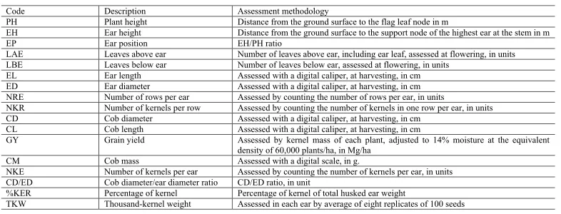
At harvesting stage, to avoid edge effects, only the two central rows were used as useful plot. Data from 17 traits (Table 1) were assessed in five representative plants (observations) of each plot. The values of these five observations composed the average of each trait for the specific plot.

Code Description Assessment methodology

PH Plant height Distance from the ground surface to the flag leaf node in m

EH Ear height Distance from the ground surface to the support node of the highest ear at the stem in m

EP Ear position EH/PH ratio

LAE Leaves above ear Number of leaves above ear, including ear leaf, assessed at flowering, in units LBE Leaves below ear Number of leaves below ear, assessed at flowering, in units

EL Ear length Assessed with a digital caliper, at harvesting, in cm ED Ear diameter Assessed with a digital caliper, at harvesting, in cm NRE Number of rows per ear Assessed by counting the number of rows per ear, in units

NKR Number of kernels per row Assessed by counting the number of kernels in one row per ear, in units CD Cob diameter Assessed with a digital caliper, at harvesting, in cm

CL Cob length Assessed with a digital caliper, at harvesting, in cm

GY Grain yield Assessed by kernel mass of each plant, adjusted to 14% moisture at the equivalent density of 60,000 plants/ha, in Mg/ha

CM Cob mass Assessed with a digital scale, in g.

NKE Number of kernels per ear Assessed by counting the number of kernels per ear, in units CD/ED Cob diameter/ear diameter ratio CD/ED ratio, in unit

%KER Percentage of kernel Percentage of kernel of total husked ear weight

TKW Thousand-kernel weight Assessed in each ear by average of eight replicates of 100 seeds

Table 1. Description of assessed traits in five plants/ears in each plot, which had composed the average of the plot.

Statistical analysis

where y is the data vector; b is the vector of plot effects within different environments (fixed); g

is the vector of genotypic effects (random); i is the vector of effects of genotype × environment (G×E) interaction (random); ε is the vector of random errors; and X, Z, and W represent the incidence matrices that fit the unknown parameters b, g, and i, respectively, to the y data vector.

Mean and variance distributions and structures

The distribution and structures of averages (A) and variances (Var) were

b g i

y =X +Z +W +

ε

_{(Equation 1)}

2 2 2

ˆ

_ˆ

0

0

ˆ

ˆ

0

_ˆ

;

0

ˆ

0

ˆ

₀

ˆ

0

0

ˆ

0

ˆ

g

i

y

Xb

_g

I

g

A

Var i

I

i

_I

ε

σ

σ

ε

σ

ε

   

_{  }



   

_{  }



   

₌

_{  }

₌



   

_{  }



   

_{ }





   

 

(Equation 2)

Mixed model equations

The model fit was obtained by the following equation of mixed model, with b estimated by the method of generalized least square and g and i predicted by BLUP.

1 2

ˆ

'

'

'

'

ˆ

'

'

'

'

ˆ

'

'

'

'

X X

X Z

X W

b

X y

Z X Z Z I

Z W

g

Z y

W X

W Z

W W I

_i

W y

λ

λ

 









 



₊



_×

₌





 









 



+











_{ }





(Equation 3) In which and 2 2 2

1 _{2 2}

ˆ

1

ˆ

ˆ

ˆ

ˆ

g g _g

c

h

h

ε

σ

λ

σ

− −

=

=

(Equation 4)

2 2 2 2 2 ₂

ˆ

1

ˆ

ˆ

ˆ

g i

c

h

c

ε

σ

λ

σ

−

−

=

=

(Equation 5)

2 2

2 2 2

ˆ

ˆ

ˆ

ˆ

ˆ

g g g i

h

ε

σ

σ

σ

σ

=

corresponds to heritability in the broad sense of the plots

2 2

2

ˆ

2 2

ˆ

ˆ

ˆ

ˆ

i g i

c

ε

σ

σ

σ

σ

=

+

+

(Equation 7)

corresponds to coefficient of determination of the G×E effects, where

σ

ˆ

2g is the genotypic

variance,

σ

_ˆ

i2 is the G×E interaction variance, and

σ

ˆ

ε2 is the residual variance.

Iterative estimators of variance components and genetic parameters by REML via

expectation-maximization algorithm

Variance components used in this study were estimated by REML using expectation-maximization algorithm (Dempster et al., 1977) according to Resende (2000):

[

]

2

ˆ

_ˆ

ˆ

'

' '

' '

' '

ˆ

( )

e

y y b X y g Z y i W y

N r x

σ

=





−

−

−





−

(Equation 8)

C22 _{and C}33 _{were derived from:}

2 2

22

ˆ ˆ

'

ˆ

ˆ

g e

g g

trC

q

σ

σ

=





+





(Equation 9)

2 2

33

ˆ' ˆ

ˆ

i e

i i

trC

s

σ

σ

=





+





(Equation 10)

1 _{11 12 13} 11 12 13

1 21 22 23

21 22 23

31 32 33 31 32 33

C

C

C

C

C

C

C

C

C

C

C

C

C

C

C

C

C

C

C

− −

















=

_

_

_{= }

_

















(Equation 11)

where C is the matrix of the coefficient of the mixed model equations, tr is the trace of a matrix operator, r(x) is the rank of the X matrix, N, q, and s are the total number of data, the number of lines, and the number of plots, respectively.

The heritability of the hybrids’ average assuming four replicates in each environment was estimated by:

where b is the number of blocks.

This expression was used to estimate the selective accuracy given by:

2

ˆ

_mg

Ac

=

_h

(Equation 13)

Genotypic correlation between hybrids and environments was estimated by:

2 2

2 2 2

ˆ

ˆ

ˆ

ˆ

ˆ

g i

ge

g i

h

r

c

σ

σ

σ

=

=

+

(Equation 14)

Genetic coefficient of variation was estimated by:

2

ˆ

₁₀₀

ˆ

g g

CV

=





σ

_µ





×









(Equation 15)

Residual coefficient of variation was estimated by:

2

ˆ

₁₀₀

ˆ

CV

ε

σ

ε

µ





=



_



_

×





(Equation 16)

where

µ

ˆ

is the average of the trait.

By using the mixed model, the predictors (REML/BLUP) of genotypic values free of the interaction were estimated by

µ

ˆ ˆ+g_i, in which

µ

^ is the overall average and gˆ_i is the genotypic values free of the G×E interaction. For the j-th environment, genotypic values (Vg) were predicted by:

Vg

=

µ

ˆ

j

+ +

g

ˆ

i

ge

ˆ

ij, where

µ

ˆ

j is the average of j-th environment; gˆi is

the genotypic effect of i-th hybrid at the j-th environment (j = 1, 2, 3 and i = 1, 2, 3, …, 15) and geˆ ij is the effect of G×E interaction regarding i-th hybrid.

Stepwise and path analysis

In order to explain the interrelationships among GY-related traits, genotypic values (Vg=µˆj+ +gˆi geˆ ij) of the 17 assessed traits (Table 1) were used in the fitting of path analysis

models. Path analysis was performed in two procedures: conventional path analysis and sequential path analysis.

Conventional path analysis

(PH, EH, EP, LAE, LBE, EL, ED, NRE, NKR, CD, CL, CM, NKE, CD/ED, %KER, and TKW) was computed, originating an X’X_16x16 matrix. Correlation coefficients of each predictor trait with GY originated an X’Y_16x1 matrix. Thus, all the 16 predictor traits were considered first-order predictors in estimating direct and indirect effects on GY. In this methodology, the direct and indirect effects (indirect effects not presented) were estimated by derivation of the system of normal equations used to estimate the multiple-regression parameters (Quinn and Keough, 2002). Thus, in order to estimate the values of β, a system of normal equations represented in the following matrix form was solved.

: : 1 :

: : 2 :

: : 16 :

1

1

1

PH EH PH TKW PH GY

EH PH EH TKW EH GY

TKW PH TKW EH TKW GY

r r r

r r r

r x r r β β β …    _…     … … … …  … …           ₌                _…   (Equation 17)

The β estimates were given by: β = (X’X)-1 _{X’Y, where β is the vector of partial regression}

coefficients (b_1,b_2,…, b_p) with p + 1 rows; (X’X)-1 _{is the inverse of X’X correlation matrix among}

predictor traits and X’Y is the matrix between each predictor trait with GY. Solving this model, it was possible to estimate the direct and indirect effects. Consider as an example the direct and indirect effects of PH on GY given by: r_PH:GY = b₁+ b₂r_PH:EH + ... + b₁₆r_PH:TKW. Where r_PH:GY is the linear correlation between PH and GY; b₁ is the direct effect of PH on GY; b₂r_PH:EH is the indirect effect of PH on GY via EH, ..., b₁₆r_PH:TKW is the indirect effect of PH on GY via TKW. Equivalent equations were fitted to the other predictors. Multiple coefficients of determination (R2_{) were}

given by: R2 _{= b}

1rGY:PH + b2rGY:EH + b3rGY:EP + β4rGY:LAE + β5rGY:LBE + β6rGY:EL + β7rGY:ED + β8rGY:NRE

+ β₉rGY:NKR + b10rGY:CD + b11rGY:CL + b12rGY:CM + b13rGY:NKE + b14rGY:DSDE + b15rGY:%KER + b16rGY:TKW

Residual effect was estimated by: 2 = 1 - R

ε .

The multicollinearity level of predictor trait matrix was measured by three measures: condition number (CN), tolerance (TOL), and variance inflation factor (VIF), as proposed by Mansfield and Helms (1982). The condition number was estimated by the ratio between the largest and smallest eigenvalue (λ) of the matrix of explanatory traits (CN = λ_Max/λ_Min). Tolerance value represented the variation of the independent trait not explained by the other independent traits of the model (

1

2

i

R

−

), where

R

2i is the coefficient of determination for the prediction of the i-th trait by the other predictor traits. The VIF values, being reciprocal of the tolerance, demonstrated the extent of the effects of other independent traits on the variance of the selected independent trait

[1/ (1

2

)]

i

R

−

, being considered the diagonal elements of (X’X)-1_{. Severe levels}

of multicollinearity were attributed to matrices with CN > 1000, and traits with VIFs > 10 and TOL < 0.1 (Mansfield and Helms, 1982).

Sequential path analysis

these traits were considered as dependent traits and stepwise regressions were carried out to estimate the second-order predictors. A sequential path diagram was presented. In order to compare the multicollinearity between the two path analysis methodologies (conventional and sequential), estimates of CN, VIF, and TOL were carried out for this methodology as described in conventional path analysis.

After the formation of sequential path diagram, path analysis was performed in sequential model, where the first-order predictors explained the interrelationships with GY and then, predictors of second-order explained the interrelationships with the first-order predictors. The direct and indirect effects were estimated as described in conventional path analysis.

Genotypic performance

Genotypic values (

µ

^_j

+ +

g ge

^_i ^ ) of GY and of the first-order predictors selected by stepwise regression were shown in graphics. In order to get a better understanding of genotypic performance, the overall average of the environment was also presented.

RESULTS

Variance components and genetic parameters

The estimates of the variance components and genetic parameters are shown in Table 2. The deviance analysis revealed significant differences (P ≤ 0.05) by the LTR test for the traits LAE, LBE, ED, NRE, GY, CM, CD/ED, and TKW, demonstrating the existence of significant differences between the full and reduced model. This is expected to single hybrids, due to narrow genetic base and quantitative traits.

The individual heritability in broad-sense (

ˆh

2g) showed values ranging from low

(0.004) to moderate magnitude (0.568) to GY and CD/ED, respectively. Low magnitude estimates were also observed for PH (0.153), LAE (0.067), LBE (0.163), EL (0.076), NKR (0.252), CL (0.118), NKE (0.246), and TKW (0.293). The heritability of genotypic mean of these traits, however, showed values of moderate (

ˆh

2mg of 0.68, 0.351, 0.529, 0.403, and 0.526

for PH, LAE, LBE, EL, and CL, respectively) to high magnitude (ˆh2mg of 0.799, 0.794, and

0.732 for NKR, NKE, and TKW).

The selective accuracy was low to GY (Ac = 0.161) and moderate to LAE (0.592) and EL (0.635). For the other traits, the accuracy was greater than 0.7, indicating that the experimental design was effective in controlling potentially disruptive effects.

CD/ED, and %KER traits, with CV_r of 1.07, 1.11, 1.22, and 1.22, respectively, indicating a possibility of selection gains for these traits.

Table 2. Variance components and genetic parameter of traits assessed in 15 hybrids grown in three environments.

*Significant by likelihood ratio test (LTR) at 5% probability error with 1 d.f. n.s._{non-significant by the LTR test.}

2 P

ˆσ

: phenotypic variance;

ˆσ

2G: genotypic variance;

ˆσ

2E: environmental variance;

ˆσ

G E2 : variance of genotype ×

environment interaction; ₂ ˆh2g: heritability of individual plots in the broad sense, i.e., the total genotypic effects; mg

ˆh : heritability of genotype average, assuming complete survival; Ac: selective accuracy assuming no loss of plots; r_ge genotypic correlation between performance at several environments; CV_g%: genotypic coefficient of

variation; CV_e%: residual coefficient of variation;

µ

ˆ

: overall average. See Table 1 for traits’ description. Trait LRT Variance components Genetic parameters

2 P

ˆσ 2

G

ˆσ 2

E

ˆσ 2

G E

ˆσ hˆ2g hˆmg2 Ac rge CVg CVe ˆ

PH 0.00n.s. _{0.023 0.004 0.019 1.25 × 10}-4 _{0.153 0.680 0.825 0.966 2.397 5.625 2.468}

EH -0.02n.s. _{0.022 0.010 0.012 1.25 × 10}-1 _{0.432 0.898 0.948 0.987 7.353 8.394 1.329}

EP -0.33n.s. _{0.002 0.001 0.001 6.30 × 10}-6 _{0.365 0.859 0.927 0.927 5.293 6.821 0.535}

LAE -5.40* 0.249 0.017 0.187 0.046 0.067 0.351 0.592 0.267 1.89 6.332 6.829 LBE -18.14* 0.451 0.074 0.241 0.136 0.163 0.529 0.727 0.350 4.402 7.975 6.159 EL -3.58n.s. _{1.591 0.121 1.247 0.223 0.076 0.403 0.635 0.351 2.286 7.353 15.187}

ED -12.61* 6.255 2.162 2.879 1.214 0.346 0.770 0.878 0.640 2.977 3.436 49.387 NRE -6.36* 2.866 1.364 1.179 0.324 0.476 0.869 0.932 0.808 7.289 6.777 16.020 NKR 0.00n.s. _{12.398 3.121 9.232 0.045 0.252 0.799 0.894 0.986 5.487 9.438 32.194}

CD -3.06n.s. _{7.012 3.620 2.915 0.477 0.516 0.900 0.949 0.884 6.568 5.893 28.970}

CL -3.44n.s. _{1.502 0.177 1.126 0.198 0.118 0.526 0.725 0.472 2.634 6.636 15.991}

GY -7.45* 2.40 × 106 _{8.63 × 10}3 _{1.89 × 10}6 _{4.99 × 10}5 _{0.004 0.026 0.161 0.017 0.900 13.309 10324.047}

CM -9.01* 37.607 17.915 14.847 4.845 0.476 0.863 0.929 0.787 17.169 15.629 24.654 NKE 0.00n.s. _{5763.02 1419.31 4315.225 28.485 0.246 0.794 0.891 0.980 7.375 12.860 510.801}

CD/ED -2.27n.s. _{1.18 × 10}-3 _{7.70 × 10}-3 _{4.47 × 10}-4 _{6.30 × 10}-5 _{0.568 0.920 0.959 0.914 4.422 3.612 0.585}

%KER -3.96* 5.227 2.906 1.951 0.370 0.556 0.910 0.954 0.887 1.950 1.598 87.415 TKW -10.78* 1869.408 548.236 958.371 362.801 0.293 0.732 0.856 0.602 6.935 9.169 337.638

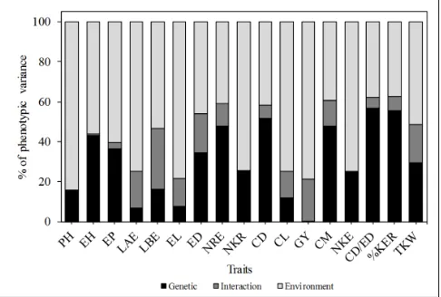
The partition of phenotypic variance into genetic, environmental, and G×E interaction variances (Figure 1) had demonstrated that only for the traits NRE, CD, CM, CD/ED, and %KER, the genotypic variance was greater than the environmental variance and G×E interaction variance. For GY, the main goal in plant-breeding programs, the phenotypic variance was largely explained: 78.80% by the environmental variance, 20.83% by the variance of G×E interaction, and only 0.36% by the genetic variance.

Conventional path analysis

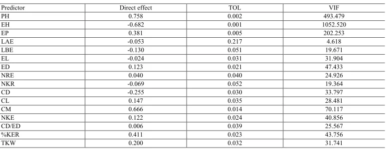
In the estimate of direct effects by the conventional path analysis method, where the 16 traits were used as first-order predictors (Table 3), high level of multicollinearity was evidenced (CN = 142,400.103). Most traits, like PH (VIF = 493.479 and TOL = 0.002), EH (VIF = 1052.52 and TOL = 0.001), and EP (VIF = 202.253 and TOL = 0.005), were highly decisive in explanation of the linear relationships. In this procedure, only LAE presented satisfactory levels of multicollinearity (VIF < 10 and tolerance > 0.1). Although R2 _{and ε}

indicated elevated fit (Table 3), the harmful effects of multicollinearity in the estimation of the path coefficients can be noticed by observing the direct effects of PH (0.758) and EH (-0.682) on GY, both with high magnitude but with opposite directions. This result is unexpected since these traits tend to be positively correlated. Thus, a reliable diagnosis of the origin of multicollinearity of the matrix of explanatory traits should be performed, and right methods must be considered aiming to adjust this problem.

Table 3. Direct effects with all traits as first-order predictors on grain yield and measures of multicollinearity

diagnosis.

Condition number = 142,400.103, R2 _{= 0.986, ε = 0.115. See Table 1 for traits’ description.}

Predictor Direct effect TOL VIF

PH 0.758 0.002 493.479

EH -0.682 0.001 1052.520

EP 0.381 0.005 202.253

LAE -0.053 0.217 4.618

LBE -0.130 0.051 19.671

EL -0.024 0.031 31.904

ED 0.123 0.021 47.433

NRE 0.040 0.040 24.926

NKR -0.069 0.052 19.364

CD -0.255 0.030 33.797

CL 0.147 0.035 28.481

CM 0.666 0.014 70.117

NKE 0.122 0.024 40.856

CD/ED 0.006 0.039 25.567

%KER 0.411 0.023 43.756

TKW 0.200 0.032 31.741

Sequential path analysis

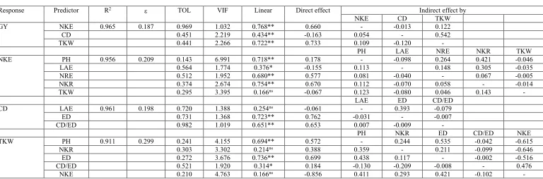
Path analysis with the second-order predictors revealed that approximately 95% of the variation of the NKE was explained by five traits, i.e., PH, LAE, NRE, NKR, and TKW. NRE and NKR had the largest positive direct effect on NKE (0.577 and 0.670, respectively), with insignificant indirect effects. Indirectly, the increase in NRE and NKR can be obtained with largest PH and largest LAE (Table 4).

Three traits (LAE, ED, and CD/ED) have explained about 96% of the variation of the CD, where ED and CD/ED had the largest direct effect (0.762 and 0.653, respectively).

Five traits (PH, NKR, ED, CD/ED, and NKE) have explained approximately 91% of the variation of the TKW. Selection for simple hybrids with higher TKW can be indirectly carried out via largest PH (0.572), NKR (0.388) and ED (0.699), and lower NKE (-0.856). The indirect effects of PH, NKR, and ED showed negative sense of moderate magnitude via NRE, indicating that plants with largest height, with largest number of kernels per row, and largest ear diameter have generally fewer kernels per ear. Thus, this interrelationship should be considered in the simultaneous search for hybrids with largest number of kernels per ear and largest thousand-kernel weight.

The diagram of sequential path analysis is shown in Figure 2. The ordering of the predictors into first- and second-order predictors had provided a better understanding of the interrelationships among grain yield-related traits.

Genotypic values

The overall average of the GY was 10.32 Mg/ha. São José do Ouro had the largest GY among the studied environments (11.95 Mg/ha), 42% higher than Viadutos and 13% higher than Santo Expedito do Sul (Figure 3). The AG8780, STATUS, and VELOZ TL hybrids showed higher GY than the average in the three environments, featuring a good genotypic stability. Conversely, the AG9045, BG7318H, and SX7331 hybrids presented GY below the average in each environment. Regarding to other hybrids, like the BM915, a differential performance was observed in each environment, characterizing a complex interaction. For this hybrid (BM915), GY was 9% smallest than the average in Santo Expedito do Sul, 8% largest than the average in São José do Ouro, showing in Viadutos GY similar to the site’s average.

Table 4. Direct and indirect effects, adjusted coefficient of determination (R2_{), noise (ε), tolerance (TOL), and} variance inflation factor (VIF) for grain yield-related traits grouped into first- and second-order predictors.

Response Predictor R2 _{ TOL VIF Linear Direct effect Indirect effect by}

NKE CD TKW GY NKE 0.965 0.187 0.969 1.032 0.768** 0.660 - -0.013 0.122 CD 0.451 2.219 0.434** -0.163 0.054 - 0.542 TKW 0.441 2.266 0.722** 0.733 0.109 -0.120 -

PH LAE NRE NKR TKW NKE PH 0.956 0.209 0.143 6.991 0.718** 0.178 - -0.098 0.264 0.421 -0.046 LAE 0.564 1.774 0.376* -0.155 0.113 - 0.148 0.305 -0.035 NRE 0.512 1.952 0.680** 0.577 0.081 -0.040 - 0.067 -0.005 NKR 0.374 2.674 0.754** 0.670 0.112 -0.070 0.058 - -0.014 TKW 0.295 3.395 0.166ns _{-0.067 0.123 -0.080 0.046 0.143 -}

LAE ED CD/ED CD LAE 0.961 0.198 0.720 1.388 0.254ns _{-0.061 - 0.393 -0.079}

ED 0.731 1.368 0.723** 0.762 -0.031 - -0.007 CD/ED 0.982 1.019 0.651** 0.653 0.007 -0.009 -

PH NKR ED CD/ED NKE TKW PH 0.911 0.299 0.241 4.155 0.694** 0.572 - 0.244 0.535 -0.042 -0.615 NKR 0.303 3.302 0.214ns _{0.388 0.359 - 0.211 -0.099 -0.646}

ED 0.272 3.676 0.736** 0.699 0.438 0.117 - -0.002 -0.516 CD/ED 0.521 1.920 0.314* 0.184 -0.130 -0.209 -0.008 - 0.476 NKE 0.210 4.763 0.166ns _{-0.856 0.411 0.293 0.421 -0.102 -}

Condition number: GY as response trait = 6.973; NKE as response trait = 32.396; CD as response trait = 3.245; TKW as response trait = 28.47. ns_{Non-significant. *},_{**Significant at 5 and 1% probability error, respectively. See}

Figure 2. Sequential path diagram illustrating the interrelationships among first- and second-order predictors

contributing to grain yield. See Table 1 for traits’ description.

Figure 3. Estimates of genotypic average for grain yield in Santo Expedito do Sul (A), São José do Ouro (B), and Viadutos (C). Horizontal lines represent the average of each environment.

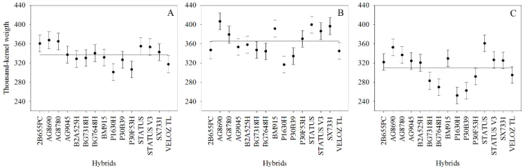
The overall average of TKW was approximately 337 g/1000 kernels. Similarly, GY and NKE in São José do Ouro had the largest average (365 g/1000 kernels). Santo Expedito do Sul showed the average equal to the overall average, while in Viadutos, the TKW was approximately 9% lower (Figure 5). AG8690, AG8780, STATUS, STATUS V3, and SX7331 hybrids were higher within the three environments. The fraction of the complex interaction was observed for this trait, coming from the different performance of 2B655PC, AG9045, B2A525H, BG7648H, BM915, and P30F53H hybrids among the environments.

Figure 4. Estimates of genotypic average for number of kernels per ear in Santo Expedito do Sul (A), São José do Ouro (B), and Viadutos (C). Horizontal lines represent the average of each environment.

Figure 5. Estimates of genotypic average for thousand-kernel weight in Santo Expedito do Sul (A), São José do Ouro (B), and Viadutos (C). Horizontal lines represent the average of each environment.

DISCUSSION

The magnitudes of CV_e observed (<16%) are similar to those found by Nardino et al. (2016), indicating good experimental quality. In other interpretation, CV_g had presented, except to GY, significant contribution to phenotypic variation, revealing the existence of genetic variation available, especially for traits with CV_g equal or greater than 1. Joint evaluation of CV_g and CV_e resulted in accuracy estimates which, according to Resende and Duarte (2007), ranged from high (0.70 < Ac < 0.90) to very high (Ac > 0.9), with the exception of LAE, EL, and GY traits.

The low estimates of

ˆh

2_g for some traits related to the plant’s morphology, e.g., PH, LAE, LBE, and EL (Table 1), revealed that these traits are highly influenced by the growing environment. This is noticed by observing the contribution of

ˆσ

2E on

ˆσ

2P (84.16, 74.98, 53.49,

and 78.40%, respectively). Low heritability values may indicate that: i) many are the genes responsible for controlling the trait’s expression; ii) a significant proportion of phenotypic variance is due to the environment or experimental error, and iii) genotypic variance is dependent on the G×E interaction (Flint-Garcia et al., 2005). As the accuracy of selection for these traits (PH, LAE, LBE, and EL) was moderate (Ac > 0.6), the experimental control was adequate, and the low values of

ˆh

2_g were attributed mainly to high

ˆσ

2E together with the

greater contribution of

ˆσ

G E2 found for these traits (Figure 1). This resulted in low r_ge values, revealing that the magnitude of these traits in an environment will not be normally observed in another environment. Oppositely, previous studies have shown

ˆh

2_g > 0.85 for PH, LAE, LBE, and EL (Flint-Garcia et al., 2005; Bello et al., 2012; Ogunniyan and Olakojo, 2014). These authors state that selection for these traits is effective. It is important to note, however, that the heritability is not a merely peculiarity of the trait, but also of the population and environmental conditions in which individuals are subjected. Since the magnitude of

ˆh

2_g is dependent on all variance components (Equation 6), the change in any of these components will be affected. Higher environmental variation tends to reduce 2

g

h

, likewise that uniform environmental conditions tend to increase it. Thus, the heritability of a trait must refer to a certain population in certain growing conditions and, even if the heritability oscillates close to zero, the trait will be inherited if this is heritable (Falconer and Mackay, 1996).

the hybrids used in this study are simple hybrids indicated for high-technology cultivation. The high environmental variation (78.80%) and, mainly of the G×E interaction (20.83%), may hinder the recommendation of simple hybrids with wide adaptability, stability, and high-yield potential, a fact that has been one of the main difficulties found by the current maize breeders (Tollenaar and Lee, 2002). Nardino et al. (2016), assessing pre-commercial maize hybrids in different locations in southern Brazil, have also shown high contribution of the environment (65%) in the phenotypic variation of GY; however, we were able to identify adapted and stable hybrids with productive potential of approximately 9.0 Mg/ha by using mixed models.

The high level of multicollinearity is out as one of the main problems in the estimates and inferential interpretation of the path coefficients (Blalock, 1963). Using the conventional method, the problems of multicollinearity of predictor traits were evident in the estimates of the regression coefficients, mainly due to the observation of unexpected direct effects of PH and EH on GY, both with high magnitudes, but with opposite directions (Table 3). Illogical direct effects (-25.90 ≤ direct effect ≤ 21.5) obtained in the presence of multicollinearity were also observed by Toebe and Cargnelutti (2013).

The high CN (142,400.103) observed in the conventional path analysis was the result of eigenvalues close to zero (see Material and Methods). Once the inversion of the matrix is required for the estimation of partial correlation coefficients, and this inversion basically depends on the division by the matrix determinant (MD), eigenvalues close to zero result in very low MD, because MD is given by the sum of products of the eigenvalues. Thus, the values in the inverse matrix become extremely sensitive to small differences in the data of the original matrix, or in other words, the inverse matrix is unstable (Quinn and Keough, 2002).

Here, we demonstrated that stepwise regressions are effective in selecting predictor traits with high-explanatory power (>90%) and minimum multicollinearity. In previous studies, multicollinearity in model of sequential path analysis was not presented (Agrama, 1996; Samonte et al., 1998). This information, however, is needed to identify the true benefit of the sequential method in comparison with the conventional method. The observation of TOL, FIV, and CN values at satisfactory levels (Table 4) demonstrated a low dependence among the chosen predictor traits, so the path coefficients could be estimated without the harmful effects of multicollinearity. The fit statistics of the models (R2 _{and ε) had values above other}

studies involving path analysis in maize and other crops (Bizeti et al., 2004; Adesoji et al., 2015; Kumar et al., 2015; Torres et al., 2015). In another way, the observation of studies that have hidden fully or partially the fit statistics from its results is worrying (Olivoto et al., 2016).

The highest grain yield of the AG8780 hybrid observed in the three environments was a result of higher number of kernels per ear and higher thousand-grain weight observed in this hybrid, which confirms the results found in path analysis. The high genetic variance and low variance of the interaction observed for GY primary’s predictors (CD, NKE, and TKW) resulted in high heritability for these traits (Table 2). Thus, indirect selection based on these traits aiming to increase the GY presents prospects of success, provided that the environmental and experimental conditions are considered by the breeder.

In conclusion, the variance components, genetic parameters, and genotypic values obtained by REML/BLUP-based procedures allow a better understanding of the performance of the traits of simple hybrids in multi-environment trials. The sequential path analysis model using the genotypic values is useful in explaining the actual interrelationships among grain yield-related traits since the environmental effects are not considered. Compared to the conventional model, the sequential path analysis model provides greater reliability when choosing predictor traits with high explanatory power and minimum multicollinearity. The joint use of REML/BLUP procedures and sequential path analysis is effective and should be considered in statistical evaluation of maize-breeding programs as well as of other worldwide-important crops.

Conflicts of interest

The authors declare no conflict of interest.

ACKNOWLEDGMENTS

The authors thank Coordenação de Aperfeiçoamento de Pessoal de Nível Superior (CAPES) for granting the Master’s scholarship for T. Olivoto. We also would like to thank Amanda Basêgio and Jaksson Klin for their valuable collaboration in conducting the field trials.

REFERENCES

Adesoji AG, Abubakar IU and Labe DA (2015). Character association and path coefficient analysis of maize (Zea mays L.). grown under incorporated legumes and nitrogen. J. Agron. 14: 158-163 http://dx.doi.org/10.3923/ja.2015.158.163. Agrama HAS (1996). Sequential path analysis of grain yield and its components in maize. Plant Breed. 115: 343-346

http://dx.doi.org/10.1111/j.1439-0523.1996.tb00931.x.

Almeida Filho JE, Tardin FD, Guimarães JF, Resende MD, et al. (2016). Multi-trait BLUP model indicates sorghum hybrids with genetic potential for agronomic and nutritional traits. Genet. Mol. Res. 15: 15017071 http://dx.doi.

org/10.4238/gmr.15017071.

Barbosa MH, Ferreira A, Peixoto LA, Resende MD, et al. (2014). Selection of sugar cane families by using BLUP and multi-diverse analyses for planting in the Brazilian savannah. Genet. Mol. Res. 13: 1619-1626 http://dx.doi.

org/10.4238/2014.March.12.14.

Baretta D, Nardino M, Carvalho IR, Oliveira AC, et al. (2016). Performance of maize genotypes of Rio Grande do Sul using mixed models. Científica 44: 403-411 http://dx.doi.org/10.15361/1984-5529.2016v44n3p403-411.

Bello OB, Abdulmaliq SY, Afolabi MS and Ige SA (2010). Correlation and path coefficient analysis of yield and agronomic

characters among open pollinated maize varieties and their F1 hybrids in a diallel cross. Afr. J. Biotechnol. 9:

2633-2639 10.4314/ajb.v9i18.

Bello OB, Ige SA, Azeez MA, Afolabi MS, et al. (2012). Heritability and genetic advance for grain yield and its component characters in maize. Int. J. Plant Res. 2: 138-145 http://dx.doi.org/10.5923/j.plant.20120205.01.

Bizeti HS, Carvalho CGP, Souza JRP and Destro D (2004). Path analysis under multicollinearity in soybean. Braz. Arch.

Blalock HM (1963). Correlated independent variables: the problem of multicollinearity. Soc. Forces 42: 233-237 http://

dx.doi.org/10.2307/2575696.

Chen L, Li YX, Li C, Wu X, et al. (2016). Fine-mapping of qGW4.05, a major QTL for kernel weight and size in maize.

BMC Plant Biol. 16: 81 http://dx.doi.org/10.1186/s12870-016-0768-6.

Dempster AP, Laird NM and Rubin DB (1977). Maximum likelihood from incomplete data via the EM algorithm. J. R. Stat. Soc. B 39: 1-38.

Falconer DS and Mackay TFC (1996). Introduction to Quantitative Genetics. 4th ed. Longmans Green, Harlow. Farrar DE and Glauber RR (1967). Multicollinearity in regression analysis: the problem revisited. Rev. Econ. Stat. 49:

92-107. http://dx.doi.org/10.2307/1937887

Flint-Garcia SA, Thuillet AC, Yu J, Pressoir G, et al. (2005). Maize association population: a high-resolution platform for quantitative trait locus dissection. Plant J. 44: 1054-1064 http://dx.doi.org/10.1111/j.1365-313X.2005.02591.x. Hallauer AR, Carena MJ and Miranda Filho JB (2010). Quantitative genetics in maize breeding. Springer, New York. Hocking RR (1976). A Biometrics invited paper. The analysis and selection of variables in linear regression. Biometrics

32: 1-49. http://dx.doi.org/10.2307/2529336

Hu X (2015). A comprehensive comparison between ANOVA and BLUP to valuate location-specific genotype effects for

rape cultivar trials with random locations. Field Crops Res. 179: 144-149 http://dx.doi.org/10.1016/j.fcr.2015.04.023. Khameneh MM, Bahraminejad S, Sadeghi F, Honarmand SJ, et al. (2012). Path analysis and multivariate factorial analyses for determining interrelationships between grain yield and related characters in maize hybrids. Afr. J. Agric. Res. 7: 6437-6446 http://dx.doi.org/10.5897/AJAR11.1581.

Kumar GP, Prashanth Y, Reddy VN, Kumar SS, et al. (2014). Character association and path coefficient analysis in maize

(Zea mays L.). Int. J. Appl. Biol. Pharm. Technol. 5: 257-260.

Kumar SVV and Babu DR (2015). Character association and path analysis of grain yield and yield components in maize (Zea Mays L.). Electron. J. Plant. Breed. 6: 550-554.

Kumar V, Singh SK, Bhati PK, Sharma A, et al. (2015). Correlation, path and genetic diversity analysis in maize (Zea mays L.). Environ. Ecol. 33: 971-975.

Mansfield ER and Helms BP (1982). Detecting multicollinearity. Am. Stat. 36: 158-160 10.1080/00031305.1982.10482818. Mohammadi SA, Prasanna BM and Singh NN (2003). Sequential path model for determining interrelationships among

grain yield and related characters in maize. Crop Sci. 43: 1690-1697 http://dx.doi.org/10.2135/cropsci2003.1690. Nardino M, Baretta D, Carvalho IRC, Olivoto T, et al. (2016). REML/BLUP in analysis of pre-commercial simple maize

hybrids. Int. J. Curr. Res. 8: 37008-37013.

Nastasić A, Jocković D, Ivanović M, Stojaković M, et al. (2010). Genetic relationship between yield and yield components

of maize. Genetika 42: 529-534 http://dx.doi.org/10.2298/GENSR1003529N.

Nataraj V, Shahi JP and Agarwal V (2014). Correlation and path analysis in certain inbred genotypes of maize (Zea mays

L.). at Varanasi. Int. J. Innov. Res. Dev. 3: 14-17.

Ogunniyan DJ and Olakojo SA (2014). Genetic variation, heritability, genetic advance and agronomic character association of yellow elite inbred lines of maize (Zea mays L.). Niger. J. Genet. 28: 24-28 http://dx.doi.org/10.1016/j.

nigjg.2015.06.005.

Oliveira EJ, Santana FA, Oliveira LA and Santos VS (2014). Genetic parameters and prediction of genotypic values for root quality traits in cassava using REML/BLUP. Genet. Mol. Res. 13: 6683-6700 http://dx.doi.org/10.4238/2014.August.28.13.

Olivoto T, Nardino M, Carvalho IRC, Follmann DN, et al. (2016). Pearson correlation coefficient and accuracy of path

analysis used in maize breeding: A critical review. Int. J. Curr. Res. 8: 37787-37795.

Piepho HP, Möhring J, Melchinger AE and Büchse A (2007). BLUP for phenotypic selection in plant breeding and variety testing. Euphytica 161: 209-228 http://dx.doi.org/10.1007/s10681-007-9449-8.

Quinn GP and Keough MJ (2002). Experimental Design and Data Analysis for Biologists. Cambridge University Press, New York.

Reddy VR, Jabeen F, Sudarshan MR and Rao AS (2012). Studies on genetic variability, heritability, correlation and path analysis in maize (Zea mays L.) over locations. Int. J. Appl. Biol. Pharm. Technol. 4: 196-199.

Resende MDV (2000). Análise estatística de modelos mistos via REML/BLUP na experimentação em melhoramento de plantas perenes. Embrapa Florestas, Colombo.

Resende MDV (2007). SELEGEN-REML/BLUP: Sistema estatístico e seleção genética computadorizada via modelos lineares mistos. Embrapa Florestas, Colombo.

Resende MDV and Duarte JB (2007). Precisão e controle de qualidade em experimentos de avaliação de cultivares.

Pesqui. Agropecu. Trop. 37: 182-194.

Samonte SO, Wilson LT and McClung AM (1998). Path analyses of yield and yield-related traits of fifteen diverse rice

Smith AB, Cullis BR and Thompson R (2005). The analysis of crop cultivar breeding and evaluation trials: an overview of current mixed model approaches. J. Agric. Sci. 143: 449-462. http://dx.doi.org/10.1017/S0021859605005587

Toebe M and Cargnelutti A (2013). Multicollinearity in path analysis of maize (Zea mays L.). J. Cereal Sci. 57: 453-462

http://dx.doi.org/10.1016/j.jcs.2013.01.014.

Tollenaar M and Lee EA (2002). Yield potential, yield stability and stress tolerance in maize. Field Crops Res. 75: 161-169. http://dx.doi.org/10.1016/S0378-4290(02)00024-2

Torres FE, Teodoro PE, Ribeiro LP, Correa CCG, et al. (2015). Correlations and path analysis on oil content of castor genotypes. Biosci. J. 31: 1363-1369. http://dx.doi.org/10.14393/BJ-v31n5a2015-26391