Tuning Exploitation and Exploration for Flower Pollination Algorithm: A Case Study on Function Optimization Problem

(1)

Tuning Exploitation and Exploration for Flower

Pollination Algorithm: A Case Study on Function

Optimization Problem

Tahsin Aziz

Ahsanullah University of Science and Technology

Dhaka-1208, Bangladesh

Md. Rashedul

Karim Chowdhury

Nafiul Nawjis

Mohammad

Shafiul Alam

ABSTRACT

Nature has exposed various progression to the researchers around the world. For solving diverse types of problems, many nature in-spired algorithms are used. Swarm Intelligence (SI) Algorithms generally evolve from the biological behavior of nature. These al-gorithms use Probabilistic search methods which is used to re-semble the behavior of biological entities. Flower Pollination Al-gorithm is one of them. Flower pollination can take place either in two ways: Global Pollination and Local Pollination. This pa-per has expa-perimented with different mix of global and local opa-pera- opera-tions to discover their optimal proportion for different uni-modal and multi-modal problems and with different search space size.

General Terms:

Algorithms, Artificial Intelligence, Genetic Algorithm, Optimization

Keywords

Meta-heuristics Algorithm, Flower Pollination Algorithm, Bioinformatics, Swarm Intelligence

1. INTRODUCTION

Optimization Problems are becoming more and more complex as they are becoming difficult to solve, even in hyper-polynomial time variants. Nature inspired optimization algorithms provide great results in comparison to other optimization algo-rithms [1] [2] [3]. Flower Pollination Algorithm is inspired by the pollination process of flowers. Pollination is the act of transferring pollen grains from the male anther of a flower to the female stigma [5]. The goal of every living organism, including plants, is to create offspring for the next generation. One of the ways that plants can produce offspring is by making seeds. Seeds contain the genetic information to produce a new plant [?].

The performance of the Flower Pollination Algorithm in terms of different probability values for exploitations and explorations is compared in this paper. This paper has designed a comparative study to identify with which probability value Flower Pollina-tion Algorithm can attain the best optimized result for different uni-modal and multi-modal problem variants.

The rest of this paper is organized as follows. Section2describes the Flower Pollination Algorithm. Section3provides details of the simulation and analysis of this algorithm having different values of probability on the benchmarking problems, parame-ter settings of the algorithms and compares their results. Finally, section4draws the outcomes of this paper with a few comments and suggestions on future research.

2. FLOWER POLLINATION ALGORITHM

2.1 Characteristics of Flower Pollination

Flowers are the agents that plants use to make their seeds. Seeds can only be produced when pollen is transferred between flowers of the same species. A species is defined a population of individuals capable of interbreeding freely with one another but because of geographic, reproductive, or other barriers, they do not interbreed with members of other species.

Flowers must rely on vectors to move pollen. These vectors can include wind, water, birds, insects, butterflies, bats, and other animals that visit flowers. Animals or insects that transfer pollen from plant to plant “pollinators” [?]. Pollinators can be very diverse. It is estimated that there are at least of two hundred thousand varieties of pollinator exist in nature.

Pollination is usually the unintended consequence of an animal’s activity on a flower. The pollinator is often eating or collecting pollen for its protein and other nutritional characteristics or it is sipping nectar from the flower when pollen grains attach themselves to the animal’s body. When the animal visits another flower for the same reason, pollen can fall off onto the flower’s stigma and may result in successful reproduction of the flower.

Pollen must be transferred from a flower’s stamen to the stigma to initialize the pollination process. When pollination occurs in the same plant then it is called self-pollination and when pollen from a plant is transferred to a different plant then that process is known as cross-pollination.

There are two types of pollination — Biotic Pollination process and Abiotic Pollination process [?] [8] [9]. In Biotic pollination, pollen is carried to the stigma by insects and animals and in Abiotic pollination, pollination occurs via wind or diffusion in water [?]. Biotic, cross-pollination may be happened in long distance. Bees, bats, birds and flies are mostly used as pollinators which are able to fly a long distance. So, these pollinators are considered as the carrier of the global pollination [?] [5].

Xin-She Yang describes this flower constancy and pollinator be-havior in the pollination process into the following four rules:

(1) Biotic and cross-pollination is considered as global polli-nation process with pollen-carrying pollinators performing L´evy flights.

(2) Abiotic and self-pollination are considered as local pollina-tion.

(2)

(4) Local pollination and global pollination is controlled by a switch probabilityp∈[0,1]. Besides the physical proxim-ity and other factors like wind and water, local pollination can have a significant fraction pin the overall pollination process.

2.2 Global Pollination and Local Pollination

The two key steps in flower pollination algorithm are: Global Pollination Process and Local Pollination Process [?]. In global pollination process, flower pollens are carried by pollinators so they may travel over a long distance because pollinators can of-ten fly and move in longer range. This global pollination can be represented mathematically as

xt+1

i =x t

i+γL(λ)(x t

i−g∗) (1)

Herext

iis the pollenior solution vectorxiat iterationt, andg∗

is the current best solution found among all solutions at the cur-rent iteration. Hereλis a scaling factor to control the step size. Hence, parameterL(λ)is also the step size which corresponds to the strength of the pollination [?] [?] [?]. Since pollinators can be travelled over a long distance with different distance steps. Here, L´evy flight can be used to mirror this travelling characteristic. AssumingL >0from a L´evy distribution

L∼ λΓ(λ)sin(πλ/2)

π

1

s1+λ, (SS0>0) (2)

Here,Γ(λ)is the standard gamma function and L´evy distribution is valid for long stepsS >0. Therefore, Rule 2 and Rule 3 which are basically for the local pollination can be represented like

xt_i+1=xt i+(x

t j+x

t

k) (3)

Here,xt

jandxtkare pollen from different flowers of the same

plant species. The equation narrates flower constancy in limited neighborhoods [?]. Assuming in mathematically ifxt

j and xtk

comes from the same species or selected from the same popula-tion, this equivalently becomes a local random walk if a graph can be drawnfrom a uniform distribution in [0,1]. The pseudo code of the flower pollination algorithm is given below.

2.3 Pseudo Code of Flower Pollination Algorithm

In reality every plant can have multiple flowers and each flower patch can release millions and billions of pollen gametes. However, to eliminate the complexity, Xin-She Yang assumed that each plant has only one flower and each flower only produce one gamete.So there is no necessity to distinguish between a pollen gamete or a flower or a plant.

For the simplicity one pollen gamete is characterised byxi. The

most fittest solution isg∗

In Algorithm 1 we have described the Flower Pollination Algo-rithm in details.

Algorithm 1 Flower Pollination Algorithm

1: Objective min or maxf(x), x= (x1, x2. . . , xd)t

2: Initialize a population of n flowers/pollen gametes with ran-dom solutions

3: Find the best solutiong∗in the initial population 4: Define a switch probabilityp∈[0,1]

5:while(t <MaxGeneration))

6: fori= 1 :n(all n flowers in the population) 7: if(rand< p)

8: Draw a (d-dimensional) step vector L which obeys a L´evy distribution

9: Global pollination viaxti+1=xti+L(g∗−xti)

10: else

11: Drawfrom a uniform distribution in [0,1] 12: Randomly choosejandkamong all the solutions 13: Local pollination viaxt+1

i =xti+(xtj−xtk)

14: end if

15: Evaluate new solutions

16: if new solutions are better, update them in the population 17: end for

18: Find the current best solutiong∗ 19:end while

3. SIMULATION AND ANALYSIS

3.1 Benchmark Functions

To evaluate that this procedure truly provides better result than the standard algorithm, we will be taking help from benchmark functions. A set of four benchmark functions suit consisting of uni-modal, multi-modal, high dimensional, low dimensional optimization functions is used by this paper and has tested whether the results have been improved or not.

A uni-modal function has only one local optimum whereas multi-modal has multiple local optima.

The search process must be able to avoid getting trapped at regions around local minima to reach global minima in multi-modal functions.

The analytical form each function, along with their names and bounds of search space of the functions are shown in Table1.

For all the functions the global minimum valuefminis 0.0. The

benchmark functions that we will be using are shown in Table 1 as follows:

3.2 Parameter Settings

The Algorithm is tested with 100 independent runs on each of the test functions listed in Table 1. The swarm size (i.e., no. of candidate solutions) is set to 25. The number of generations is set to 1000, 1500 and 2000 for D = 10, 30 and 50 respectively for each run. We have used probability valuepas 0.1, 0.2, 0.3, 0.4, 0.5, 0.6, 0.7 and 0.9 in the simulation.

3.3 Experimental Results

For any swarm intelligence algorithm, there should be a coor-dination between the degrees of explorations and exploitations with which the swarm members search across the search space.

(3)

Table 1. : Benchmark functions used in the experimental studies. Here, D: Dimensionality of the Function, S: Search Space, C: Function Characteristics with Values — U: Uni-modal and M: Multi-modal.For all the functionfmin= 0.0

Function No Function Name D C S Function Definition

f1 Rastrigin 10,30,50 M [−15,15]D f1(x) = 10d+

Pd

i=1(x2i−10cos(2πxi))

f2 Sphere 10,30,50 U [−5.12,5.12]D f2(x) =P

d i=1x

2

i

f3 Zakharov 10,30,50 U [−5,10]D f3(x) =Pdi=1xi2+ (Pdi=10.5ixi)2+ (Pdi=10.5ixi)4

f4 Michalewicz 10,30,50 M [0, π]D f4(x) =−

Pd

i=1sin(xi)sin2m( ix2

i

π )

Flower Pollination Algorithm controls the degrees of explo-rations and exploitations with a switch probability p. In FPA the global and local pollination technique is used to balance between explorations and exploitations.

In global pollination, the L´evy distribution is applied to generate new solutions; while in local pollination new solutions are generated using randomly selected local solutions. The L´evy distribution has the capability to generate new solutions with bigger mutation step size. Thus the algorithm is more likely to escape from the locally optimal points.

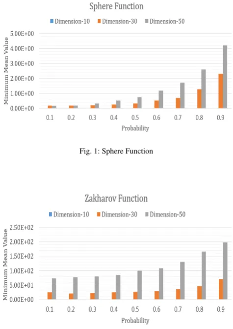
For simulation, four benchmark functions have been used in this experiment. Among them Sphere Function and Zakharov Function are uni-modal and Rastrigin Function and Michalewicz Function are multi-modal. In Table 2 and Table 3 , it can be seen that the solution quality (mean value) is much better for Probability values lower for the uni-modal function and higher for the multi-modal function. Also the probability decreases inversely with the dimension can be observed by the values of this tables.

In this paper, the values of minimum mean with reference to probability in different dimensions for the four functions is plotted to gather some knowledge in which values of p the functions gives the best result.

For uni-modal functions,

Figure 1 shows that the value offminincreases with the increase

of probability.So it may be expected that the best result may be obtain from probability value 0.1.

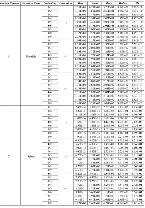
Figure 2 shows that the value of fmin decreases with the

increase of probability upto it reaches a neighbouring area of probability 0.5 for dimension 10 and dimention 30.But for dimension 50 the value offminincreases with probability.So

the best result may be obtained from probability value 0.5 for dimension 10 and dimension 30 and for dimension 50 the value ofpmay be 0.1 to 0.4 to obtain the best result can be expected. For multi-modal functions,

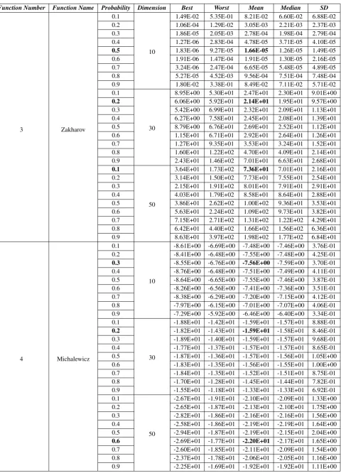
Figure 3 shows that the value of fmin decreases with the

increase of probability upto it reaches a neighbouring area of probability 0.5. After that it starts increasing again with the

Fig. 1: Sphere Function

Fig. 2: Zakharov Function

probability. So the best result may be obtain from probability value 0.5.

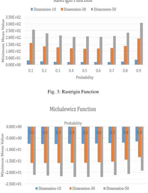
Figure 4 shows that the value offmindecreases with the increase

(4)

Table 2. : Comparison of Probabilitypused in FPA on four standard benchmark functions. Algorithms are run 100 different times on each of the functions. The best result for each probability with each dimensionality is marked with boldface font.

Function Number Function Name Probability Dimension Best Worst Mean Median SD

1 Rastrigin

0.1

10

1.75E+01 6.21E+01 3.20E+01 3.14E+01 7.86E+00 0.2 1.16E+01 4.89E+01 2.60E+01 2.56E+01 6.69E+00 0.3 1.34E+01 3.47E+01 2.25E+01 2.18E+01 5.11E+00 0.4 9.36E+00 3.34E+01 2.03E+01 1.95E+01 4.95E+00 0.5 1.00E+01 3.46E+01 2.03E+01 1.91E+01 5.23E+00 0.6 9.62E+00 3.15E+01 2.01E+01 2.01E+01 5.09E+00 0.7 1.18E+01 3.05E+01 2.03E+01 1.95E+01 4.44E+00 0.8 1.12E+01 3.52E+01 2.37E+01 2.31E+01 4.95E+00 0.9 2.27E+01 5.56E+01 3.81E+01 3.76E+01 6.49E+00 0.1

30

50

1.64E+02 3.50E+02 2.59E+02 2.57E+02 3.80E+01 0.2 1.47E+02 3.19E+02 2.30E+02 2.30E+02 3.26E+01 0.3 1.34E+02 3.09E+02 2.15E+02 2.14E+02 3.32E+01 0.4 1.38E+02 2.65E+02 2.06E+02 2.07E+02 2.73E+01 0.5 9.23E+01 2.82E+02 2.08E+02 2.09E+02 3.06E+01 0.6 1.51E+02 2.83E+02 2.05E+02 2.01E+02 2.87E+01 0.7 1.36E+02 2.80E+02 2.12E+02 2.09E+02 2.67E+01 0.8 1.76E+02 3.11E+02 2.37E+02 2.37E+02 2.82E+01 0.9 2.45E+02 3.79E+02 3.08E+02 3.07E+02 2.73E+01

2 Sphere

0.1

10

2.45E-04 1.30E-02 2.57E-03 2.13E-03 1.75E-03 0.2 3.29E-05 8.31E-04 1.68E-04 1.33E-04 1.35E-04 0.3 4.14E-06 1.08E-04 2.12E-05 1.64E-05 1.76E-05 0.4 1.02E-06 6.47E-05 6.98E-06 4.30E-06 9.67E-06 0.5 1.55E-07 1.31E-05 2.47E-06 1.72E-06 2.12E-06 0.6 2.53E-07 1.63E-05 2.68E-06 1.95E-06 2.73E-06 0.7 7.02E-07 4.65E-05 9.02E-06 6.35E-06 8.13E-06 0.8 1.44E-05 5.81E-04 1.46E-04 1.18E-04 1.09E-04 0.9 1.99E-03 2.84E-02 1.08E-02 9.21E-03 5.87E-03 0.1

30

6.30E-02 4.22E-01 1.97E-01 1.78E-01 8.21E-02 0.2 5.63E-02 6.90E-01 1.93E-01 1.78E-01 1.06E-01 0.3 3.07E-02 6.09E-01 2.15E-01 2.00E-01 1.10E-01 0.4 4.60E-02 8.45E-01 2.72E-01 2.23E-01 1.63E-01 0.5 6.76E-02 1.37E+00 3.38E-01 2.85E-01 2.21E-01 0.6 1.47E-01 1.75E+00 5.37E-01 4.97E-01 2.90E-01 0.7 1.17E-01 1.81E+00 6.96E-01 5.91E-01 3.63E-01 0.8 3.73E-01 3.07E+00 1.29E+00 1.14E+00 6.36E-01 0.9 6.50E-01 4.73E+00 2.31E+00 2.17E+00 8.02E-01 0.1

50

(5)

Table 3. : Comparison of Probabilitypused in FPA on four standard benchmark functions. Algorithms are run 100 different times on each of the functions. The best result for each probability with each dimensionality is marked with boldface font.

Function Number Function Name Probability Dimension Best Worst Mean Median SD

3 Zakharov

0.1

10

1.49E-02 5.35E-01 8.21E-02 6.60E-02 6.88E-02 0.2 1.06E-04 1.29E-02 3.05E-03 2.21E-03 2.37E-03 0.3 1.86E-05 2.05E-03 2.78E-04 1.98E-04 2.79E-04 0.4 1.27E-06 2.83E-04 4.78E-05 3.71E-05 4.10E-05 0.5 1.83E-06 9.27E-05 1.66E-05 1.26E-05 1.49E-05 0.6 1.91E-06 1.47E-04 1.91E-05 1.30E-05 2.16E-05 0.7 3.24E-06 2.47E-04 6.65E-05 5.48E-05 4.89E-05 0.8 5.27E-05 4.52E-03 9.56E-04 7.51E-04 7.48E-04 0.9 1.80E-02 3.38E-01 8.49E-02 7.11E-02 5.71E-02 0.1

30

50

3.64E+01 1.73E+02 7.36E+01 7.01E+01 2.16E+01 0.2 3.14E+01 1.50E+02 7.73E+01 7.55E+01 2.54E+01 0.3 2.15E+01 1.91E+02 8.01E+01 7.91E+01 2.91E+01 0.4 4.03E+01 1.79E+02 8.58E+01 8.64E+01 2.88E+01 0.5 3.86E+01 2.62E+02 1.00E+02 9.36E+01 3.53E+01 0.6 5.63E+01 2.24E+02 1.09E+02 9.73E+01 3.82E+01 0.7 7.15E+01 2.71E+02 1.31E+02 1.22E+02 4.29E+01 0.8 6.42E+01 4.40E+02 1.66E+02 1.56E+02 6.36E+01 0.9 8.63E+01 3.97E+02 1.98E+02 1.77E+02 6.84E+01

4 Michalewicz

0.1

10

-8.61E+00 -6.69E+00 -7.48E+00 -7.46E+00 3.76E-01 0.2 -8.41E+00 -6.48E+00 -7.55E+00 -7.48E+00 4.25E-01 0.3 -8.55E+00 -6.76E+00 -7.56E+00 -7.59E+00 3.70E-01 0.4 -8.76E+00 -6.48E+00 -7.51E+00 -7.49E+00 4.11E-01 0.5 -8.64E+00 -6.65E+00 -7.55E+00 -7.46E+00 3.87E-01 0.6 -8.26E+00 -6.56E+00 -7.41E+00 -7.36E+00 3.51E-01 0.7 -8.38E+00 -6.29E+00 -7.20E+00 -7.15E+00 4.12E-01 0.8 -7.97E+00 -6.15E+00 -7.01E+00 -7.07E+00 4.06E-01 0.9 -7.29E+00 -5.92E+00 -6.46E+00 -6.40E+00 3.34E-01 0.1

30

-1.88E+01 -1.42E+01 -1.59E+01 -1.57E+01 8.88E-01 0.2 -1.82E+01 -1.43E+01 -1.59E+01 -1.58E+01 8.46E-01 0.3 -1.89E+01 -1.40E+01 -1.59E+01 -1.57E+01 9.68E-01 0.4 -1.77E+01 -1.37E+01 -1.57E+01 -1.57E+01 8.65E-01 0.5 -1.87E+01 -1.36E+01 -1.57E+01 -1.56E+01 1.05E+00 0.6 -1.83E+01 -1.35E+01 -1.56E+01 -1.55E+01 1.00E+00 0.7 -1.84E+01 -1.35E+01 -1.52E+01 -1.51E+01 8.75E-01 0.8 -1.70E+01 -1.28E+01 -1.45E+01 -1.44E+01 7.82E-01 0.9 -1.55E+01 -1.18E+01 -1.33E+01 -1.33E+01 6.92E-01 0.1

50

(6)

Fig. 3: Rastrigin Function

Fig. 4: Michalewicz Function

4. CONCLUSION

This paper presents a comparative study between different values of the switch probabilitypin flower pollination algorithm. This algorithm uses swarm intelligence to find the global optimum value of the continuous optimization problems. Numerical re-sults on the standard benchmark problems for Flower Pollination algorithms demonstrate the effectiveness and competitiveness of the algorithms based on the value ofp. There has been a few re-search works that try to improve the performance of the Flower Pollination Algorithm. In future the plan is to compare with those algorithms with the Flower Pollination Algorithm with modified switch probability with a conjecture to obtain better results.

5. REFERENCES

[1] Y. Xin-She, “Engineering Optimization: An Introduction with Metaheuristic Application,” Wiley, 2010.

[2] H. A. Abbass and R. Sarker, “The Pareto diffential evo-lution algorithm,” Int. J. Artificial Intelligence Tools, vol. 11(4), pp. 531-552, 2002.

[3] Y. Xin-She,“Nature-inspired Metaheuristic Algorithms,” Luniver Press, 2008.

[4] Y. Xin-She, K. Mehmet and H. Xingshi, “Multi-objective Flower Algorithm for Optimization,” in International Con-ference on Computational Science, ICCS 2013, 2013. [5] M. Walker, “How flowers conquered the world,” BBC

Earth News, 10 July 2009.

[6] Y. Xin-She, “Flower pollination algorithm for global opti-mization,” Unconventional Computation and Natural Com-putation, Lecture Notes in Computer Science, vol. 7445, p. 240–249, 2012.

[7] K. Gaganpreet and D. S. Dr., “Pollination Based Optimiza-tion or Color Image SegmentaOptimiza-tion,” InternaOptimiza-tional Journal of Computer Engineering and Technology (IJCET), vol. 3, no. 2, pp. 407-414, July-September 2012.

[8] K. S, “Pollination based optimization,” in 6th International Multi Conference on Intelligent Systems, Sustainable, New and Renewable Energy Technology and Nanotechnology (IISN2012), March 16-18,2012.

[9] N. Waser, “Flower constancy: definition, cause and mea-surement,” The American Naturalist, 1986.