Centroid Based Localization Utilizing Artificial Bee Colony Algorithm

RESEARCH ARTICLE

Centroid Based Localization Utilizing Artificial Bee

Colony Algorithm

Vikas Gupta

Chandigarh Engineering College, Landran, Mohali, Punjab, India.

[email protected]

Brahmjit Singh

National Institute of Technology, Kurukshetra, Haryana, India.

[email protected]

Published online: 27 June 2019

Abstract – Estimation of position of unknown nodes is of immense importance for proper deployment and tracking of sensors. The centroid based localization algorithm (CLA) is widely used for the localization of the sensors but its original and modified versions suffer from large positioning error. Here the localization algorithm is evaluated in terms of localization error utilizing artificial bee colony based (ABC) algorithm. Comparison of outcome is presented through other widely used techniques including swarm based particle swarm optimization (PSO) and evolutionary algorithms based differential evolution (DE) on basic centroid localization algorithm. The results obtained through simulation demonstrate that localization error is minimal in ABC and DE based CLA as compared to basic and PSO based schemes but the computation time is the largest in DE based localization algorithm as compared to others. In comparison to the basic CLA the average localization error is reduced by 95% and computation time is increased by seven fold in ABC based CLA. It may be established that having considered localization error of prime importance, ABC algorithm based CLA is the most suitable strategy for localization amongst all the three algorithms.

Index Terms – Wireless Sensor Networks, Localization, Artificial Bee Colony, Particle Swarm Optimization, Differential Evolution, Localization Error etc.

1. INTRODUCTION

Estimation of unknown positions of sensor nodes distributed arbitrarily in the area of concern is termed as localization and is of immense significance. Localization plays a significant role in location of sensed events, geographic routing and target tracking [1]. Broadly the location estimation algorithms are separated in two classes, namely range based and range free. Time of arrival (TOA) [2], time difference of arrival (TDOA) [3], angle of arrival (AOA) [4], and received signal strength indicator (RSSI) [5] are generally utilized algorithms those fall in the class of range based. In order to localize the nodes these algorithms rely on accurate point-to-point assessment of position. The major benefit of these range based algorithms is that they locate the position of

unidentified sensor nodes with good correctness, but the kind of hardware these techniques use is very costly. However, the range free location determination algorithms do not involve such kinds of hardware for localization. They find the locations of unidentified nodes by means of connectivity information and hence entire arrangement is localized. A hefty amount of research papers on range free localization methods have been published in literature. For example, Bulusu et al. in [6] presented a centroid based location estimation algorithm that falls under the category of range free algorithms. In this work, the receiver localizes itself to the areas, which coincide with the area of the anchor nodes. The coinciding area is called as the centroid of the anchor nodes. Beacon nodes or reference nodes are the other names of anchor nodes used in literature. The beacon nodes or the beacons are having some built in location determination equipment. Hop count based localization algorithm DV-HOP was presented by Niculescu et al. in [7]. The notion of this algorithm was to replace the Euclidean distance between two nodes with inter node hop distance. Another range free algorithm, APIT (approximation point in triangulation test) was proposed by He et al. in [8]. Here three beacon nodes create triangular regions; the centroid formed by the intersection of these regions is used to find out the position of unknown sensor nodes.

RESEARCH ARTICLE

different bio inspired and evolutionary algorithms based soft computing techniques have been proposed in past by the research community. Some of the utilized techniques reported in literature are genetic algorithm [11], simulated annealing [11], artificial neural networks [12][13], fuzzy logic systems [14], particle swarm optimization (PSO) [14][15]16][17][18][19], differential evolution [20] etc. In general, all these algorithms optimize the research problem by considering one or more parameters. For example in PSO [14] the interest is to optimize the objective function and in the problem of localization the target is to minimize the localization error. In [21] the differential evolution algorithm is applied on RSSI (received signal strength indicator) to optimize the location estimation of the unknown sensor nodes.

In [14] the RSSI from reference nodes to the unidentified nodes is taken in terms of weights and weights are optimized using fuzzy inference engine. These optimized weights further improve the average localization error. Use of these soft computing techniques by the research community to optimize the positioning error motivates us to use ABC algorithm. So in this research article, the original centroid localization algorithm (CLA) is examined and its performance is evaluated using ABC algorithm. Further, the same algorithm is first studied with swarm intelligence based PSO algorithm, then with evolutionary algorithm based DE algorithm, and a comparison of these algorithms is made. Remaining structure of paper is separated into 5 sections. Related work in detail is presented in section 2. Simulation of ABC based CLA is given in section 3. Section 4 discuss in detail the results and discussion. Conclusions followed by references are presented in section 5.

2. RELATED WORK 2.1. Basic Centroid Localization Algorithm

In [6] Bulusu et al. presented an idealized connectivity based model for outdoor propagation under uncluttered environment. They assumed equal power for all the nodes. In this model the reference are put on known locations. The unknown nodes localize themselves in the region that coincides with the region of intersection of the anchors. They estimated the position of unknown sensor nodes using equation 1 [6].

(𝑋𝑒𝑠𝑡, 𝑌𝑒𝑠𝑡) = (𝑋𝑖1+𝑋𝑖2_𝑘+⋯+𝑋𝑖𝑘,𝑌𝑖1+𝑌𝑖2_𝑘+⋯+𝑌𝑖𝑘) (1)

Here (Xest, Yest) is the estimated value of unknown

coordinates of sensor node and the number k represents the amount of reference nodes. The performance measure used to determine the accuracy of this method called as localization error (LE) can be described with the equation 2 [6].

𝐿𝐸 = √(𝑋𝑒𝑠𝑡− 𝑋𝑎)2+ (𝑌𝑒𝑠𝑡− 𝑌𝑎)2 (2)

Here (Xa, Ya) depicts the actual values of coordinates of

unidentified sensor node. This algorithm is very easy and inexpensive but the main disadvantage associated with this algorithm is large localization error. This error in this scheme comes out to be within 2 to 4 meters. An improved version of the original CLA algorithm is presented in [22]. Hay-qing et al. premeditated the coordinates of unknown node on the basis of weights. They estimated the distance between transmitting and receiving node and decided the weights based on these distances. The estimated value of the unknown coordinates is calculated based on the equation 3 [22].

(𝑋𝑒𝑠𝑡, 𝑌𝑒𝑠𝑡) = (𝑤1∗𝑋_𝑤1+⋯+𝑤𝑛∗𝑋𝑛

1+⋯+𝑤𝑛 ,

𝑤1∗𝑌1+⋯+𝑤𝑛∗𝑌𝑛

𝑤₁+⋯+𝑤_𝑛 ) (3)

The weights are calculated using RSSI. This method increases the accuracy level but achievement of this improved algorithm extremely depends upon the optimization of these weights which is a tedious task. Blumenthal et al. [23] presented a weighted centroid algorithm for the estimation of position of unknown sensor nodes. They investigated the theoretical and practical aspects of RSSI measurements and studied the impact on localization error. Although the localization error obtained from this method is less than 1 m but one of the disadvantages of this method is that it do not take into account the environmental abnormalities while estimating the unknown coordinates. Quande et al. [24] proposed a weight compensated RSSI based weighted CLA. The algorithm is simple to implement consume less power and increases the accuracy of localization compared to other weighted CLAs. Although the localization error is reduced to 2.81 m but still the localization error is too big which need to be reduced further. Therefore, the sole objective of present research is to optimize the localization error of basic centroid based algorithm.

2.2. Natural Behavior of Honey Bees

RESEARCH ARTICLE

again. General architecture of algorithm of ABC may be described as [25]

Repeat

Employed Bee (EBs) stage Onlooker Bees (OBs) stage Scout Bees (SBs) stage Remember the optimized result obtained Until (the threshold reaches)

2.2.1. Localization Using ABC Algorithm

The ABC algorithm [25][26][27] comes under the category of swarm intelligence based soft computing technique that uses the food finding activities of honey bees to optimize the solution. In the context of localization problem, all food sources represent all the sensors nodes scattered in the area of interest. The degree of sweetness or nectar present in the food source gives the level of suitability of the outcome. To get the optimized value of localization error, it is considered as the objective function. The control parameters are decided and scout bees (SBs) initialize the inhabitants of food references (or solutions). In first phase the EBs hunt for all new available food references having large nectar present in the vicinity of the these references. Every time after discovering the new food references, the greedy selection algorithm between new obtained solution and its parent is used to obtain new fitness value. This food references information is conveyed by the EBs with OBs waiting in the hive with the help of a dance on the dancing area. Based on the knowledge given by the EBs, the OBs select their food probabilistically for which fitness selection method, roulette wheel selection is employed. The sources that are poor or exploited are deserted and scout bees start to seek new solutions. These steps are replicated repeatedly in anticipation of a threshold.

2.2.2. Initialization of Population

Initially, the artificial bee colony algorithm produces inhabitants of evenly distributed solutions where each solution xi (i = 1, 2... N) depicts a d-dimensional vector. Here

xi represents the ith food source and d signifies the variables

present in the problem of optimization. Generation of each food source can be presented by the given equation 4 [27].

𝑥𝑖𝑗 = 𝑥min 𝑗+ 𝑟𝑎𝑛𝑑[0,1](𝑥max 𝑗− 𝑥min 𝑗) (4)

Where xmin j is the lower and xmax j is the upper restriction of xi

in the jth direction.

2.2.3. Employed Bees Phase

Here the existing solution is modified on the basis of its fitness value. Depending upon the worth of fitness of fresh solution, the bees update their position with newer value and

discard the older ones. This position updation is represented by equation 5 [27].

𝑣𝑖𝑗= 𝑥𝑖𝑗 + 𝜙𝑖𝑗(𝑥𝑖𝑗− 𝑥𝑘𝑗) (5)

Where 𝜙_𝑖𝑗(𝑥_𝑖𝑗− 𝑥_𝑘𝑗) is called as step size, k Є {1, 2...N} and j Є {1, 2... d} are two arbitrarily selected indices. And k and i are chosen to be of different values so as to have some significant contribution of step size, 𝜙_𝑖𝑗 whose value lies in between [–1, 1].

2.2.4. Onlooker Bees Phase

In OBs phase, the suitability of updated solutions and the positional data are shared with OBs present in hive. These bees analyses existing knowledge and pick a resolution based on some probability. This probability (Pi) is given by equation

6 [27].

𝑃𝑖=_∑ 𝑓𝑖𝑡_𝑓𝑖𝑡𝑖 𝑖 𝑁

𝑖=1 (6)

Where 𝑓𝑖𝑡𝑖 is the worth of fitness for the ith solution.

2.2.5. Scout Bees Phase

In SBs, if solutions obtained by the employed bees cannot be enhanced further even after a predetermined threshold, the employed bees now become the scouts and current solutions obtained by them are discarded. The scouts again begin moving arbitrarily in the hunt for new sources (or solutions). The preset number of cycle or the limit of rejection is an important control parameter. Let us suppose that the discarded solution is x, the scout bees replace this source (solution) with newer on the basis of equation 7[27]

𝑥_𝑖𝑗= 𝑥_𝑚𝑖𝑛𝑗 + 𝑟𝑎𝑛𝑑[0,1](𝑥𝑚𝑎𝑥𝑗 − 𝑥𝑚𝑖𝑛𝑗 ), ∀𝑗= 1,2, … 𝑑 (7)

Where and are the lower and upper restrictions of in jth direction.

2.3. Particle Swarm Optimization

RESEARCH ARTICLE

particle and the global best (gbest) is the collective best considered among all the particles. Updation of velocity and position is done using the equation 8 and 9.

𝑣𝑖(𝑡 + 1) = 𝑤. 𝑣𝑖(𝑡) + 𝑐1. 𝑟𝑎𝑛𝑑(). (𝑃𝑝𝑏𝑒𝑠𝑡(𝑡) −

𝑥𝑖(𝑡)𝑐2. 𝑟𝑎𝑛𝑑(). (𝑃𝑔𝑏𝑒𝑠𝑡(𝑡)𝑥𝑖(𝑡)) (8)

𝑥𝑖(𝑡 + 1) = 𝑥𝑖(𝑡) + 𝑣𝑖(𝑡 + 1) (9) In the above equations xi (t + 1) is the updated new position

and vi (t + 1) is the updated new velocity. Another important

factor w represents the weight assigned to the first part of the equation 8, w.vi (t) which is termed as the inertia term. The

succeeding part of the equation 8 that represents the individual behavior of the particle is called as cognition part and third part that represents the collective behavior of the particles is called as the social part. In both parts, c1 and c2 are acceleration coefficients which are constant terms. Here the localization error (equation 2) is taken as the objective function and the optimized localization error is determined using PSO.

2.4. Differential Evolution

In localization of unknown nodes in wsn, the problem of localization is taken as the problem of differential evolution and the optimized solution is found. Like genetic algorithm the differential evolution algorithm is also an algorithm which is based on population that employs the same operators: crossover, mutation and selection [20][21][29][30]. In general, the genetic algorithm relies on crossover whereas the DE relies on mutation. The mutation is given importance as it gives good parametric variations and diverse results. The equation of mutation is given by

𝑀𝑡𝑚𝑢𝑡𝑎𝑡𝑒𝑑= 𝑀𝑏𝑒𝑠𝑡+ 𝑆 ∗ (𝑇𝑣− 𝑅𝑣) (10)

Where Mbest is the best solution, Mt is the mutated value, S is

the scaling factor and TV and RV are the targeted and

randomly selected positions. Here also the localization error is considered as fitness function of DE and the optimum fitness function is found by mutation (equation 10), cross over and selection.

3. SIMULATION OF ABC BASED CENTROID LOCALIZATION ALGORITHM

In wireless sensor networks (wsn) the problem associated with the localization is the error in estimation of exact coordinates of the unknown nodes. Here first the basic CLA is studied and simulated in matlab and then localization error is premeditated by estimating the distinction between actual and estimated values of coordinates of unidentified sensor nodes. To reduce the error in CLA based algorithm a big number of swarm based soft computing techniques have been proposed in past. But very little work has been done using ABC algorithm which is a very good optimization algorithm and extensively used method to find the optimum solutions of

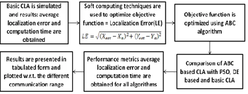
many problems. So here ABC algorithm is applied on centroid based algorithm for diverse values of an important network parameter, the communication range. So in the present work the effects of swarm based technique ABC on localization error in wsn are studied. In algorithm of ABC best position of food source denotes the best possible solution in the problem of optimization. While using the ABC algorithm in wsn each food resource represents the distribution of sensors in the area of interest and the amount of nectar present in the food resource shows the height of fitness of the solution. And localization error that is to be optimized (given in equation 2) is considered as the objective function. The goal of the bees in ABC algorithm is to unearth the best possible solution and three categories of the bees namely the EBs, OBs and the SBs fulfill this goal. The EBs exploits the food source and shares this knowledge with the OBs. In terms of localization problem the best position is determined by the employed bees using equation 5. The onlooker bees evaluate this sweetness (nectar) information using certain threshold. For localization problem this is the probability given in equation 6 which acts as threshold. The onlooker bees become the scout bees after all the nectar is exhausted or if the quality of nectar is below the threshold. These scout bees again start searching the newer food source using equation 7. The minimum localization error is the best solution achieved from the ABC algorithm. The proposed approach, in very simplified manner is presented here with the help of an architectural diagram as shown in the Figure 1. It can be easily understood from the diagram that approach starts with simulation of basic centroid based localization algorithm (CLA). Due to the large localization error in CLA, soft computing techniques are employed to reduce or optimize this error. For doing so the localization error is assumed as the objective function to be optimized. Then ABC algorithm is used on basic CLA and results obtained are compared with PSO and DE based CLA.

Figure 1 An Architectural Diagram of the Proposed Approach

RESEARCH ARTICLE

pseudocode for the whole ABC based centroid localization algorithm is presented in sub section 3.1.

3.1. Pseudocode of ABC based CLA

The pseudocode 1 represents the ABC based CLA. Objective function (equation 2)

Initialize food source or solutions N (equation 4) Cycle=1;

While cycle <= Maximum Threshold Do Begin

Employed bees’ phase For i=1 to N

Generate a candidate solution vi for xi and evaluate 𝑣𝑖𝑗 from

𝑥𝑖𝑗 (equation 5)

If fitness of vi > xi Then swap values

Counter (i) =0

Else counter (i) = counter (i) + 1 End #of employed bees Exit from loop if best found Onlooker bees’ phase While i<=N

If fitness of random solution < p (probability)

Generate candidate solution vi for xi (using equation 5)

If fitness of vi > xi Then swap values

Counter (i) =0

Else counter (i) = counter (i) + 1 Exit from loop if best found If i=N+1

Scout bees’ phase

Solution with best value at threshold

Solution is changed with new random solution (equation 7) Cycle = cycle +1

End while

Pseudocode 1 ABC based CLA 4. RESULTS AND DISCUSSION

All the network parameters with numerical values used for the simulation of basic CLA and ABC based CLA are presented in the table 1. The table 1 contains the summary of

the parameters chosen and mathematical values used for the simulation environment. All the terms used in the table 1 are self-explanatory. As indicated in table 1 an area of 100 sqm is considered and 200 sensor nodes are spread arbitrarily in this area. As the coordinates of these unknown nodes in centroid based localization is estimated on the basis of some anchor nodes so in the same area of 100sqm 40 anchor nodes (the nodes having GPS like arrangements) are also randomly distributed. That means the anchor ratio chosen is .2 (anchor nodes divided by the total number of nodes). The communication range is varied from 10m to 100m. The path loss model considered for simulation is log normal multiplicative. The path loss exponent value is chosen to be 2. Performance measures the average localization error and computational time is obtained after simulation in matlab. All the numerical figures mentioned in the paper related to the results are obtained by taking the average of all the values (given in table 2 and 3) with respect to the communication range which varies from 10m to 100m. The average localization error and computation time obtained through simulation of ABC based CLA, PSO based CLA, DE based CLA and basic CLA with respect to the different communication range is given in subsection 4.1 and 4.2.

Parameter Setting of the value

Area of interest 100×100 m2

Number of nodes 200 Anchor nodes 40 Communication range 10-100m

Path loss exponent 2

Path loss model Log normal multiplicative Anchor ratio 0.2

Table: 1 System Parameters

Communic ation Range (m)

Average Localiza tion Error (LE) in ABC based CLA (m)

Average Localiza tion Error (LE) in PSO Based CLA (m)

Average Localiza tion Error (LE) in DE based CLA (m)

RESEARCH ARTICLE

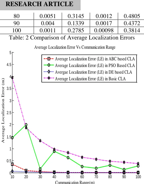
80 0.0051 0.3145 0.0012 0.4805 90 0.004 0.1339 0.0017 0.4372 100 0.0011 0.2785 0.00098 0.3814 Table: 2 Comparison of Average Localization Errors

Figure 2 Average Localization Error for Various Values of Communication Range

4.1. Average Localization Error for Different Communication Range:

Table 2 presents all the values of average localization error for ABC, PSO, DE based CLA and basic CLA obtained after simulation for diverse values of communication range. Figure 2 shows the graphical illustration of average localization error for all of the localization algorithms. It can be shown from the graph that the localization error is largest in basic centroid based algorithm that reduces by using PSO but still the error is large. This error further reduces by using the ABC and DE algorithms. The performance of these two algorithms is largely same for localization error. One of the common observations for all of the algorithms is that there is an inverse relation between communication range and localization error. It can also be concluded from the observation that the average localization error reduces by 95% in ABC based CLA, 45% in PSO based CLA and 99% in DE based CLA in comparison to basic CLA.

4.2. Computation Time for Different Communication Range: The computation time taken in simulations of ABC, PSO, DE based CLA and basic CLA in matlab, for different communication ranges is presented in table 3. Figure 3 shows the graphical illustration of computation time for all of the four localization algorithms. It can be shown from the plot

that the computation time is smallest in basic centroid based algorithm which suffers from large localization error. This computation time increases with PSO at same time localization error decreases. The computation time is largest for DE based algorithm although the localization error is very small. For ABC based algorithm the computation time is very small as compared to the DE based CLA although the localization error for both is approximately same. It can also be concluded from the observation that the computation time increases to seven fold in ABC based CLA, three fold in PSO based CLA and thirty fivefold in DE based CLA if compared with original CLA.

Communi cation Range (m) Comput ation Time in ABC based CLA(se conds) Computat ion Time in PSO Based CLA (seconds) Computat ion Time in DE based CLA (seconds) Comput ation Time in Basic CLA (second s) 10 46.925 21.521 240.74 6.851 20 47.097 21.171 238.152 6.87 30 46.983 21.122 240.432 6.831 40 46.864 21.348 239.693 6.876 50 47.711 21.889 241.171 6.874 60 47.724 22.198 244.233 6.973 70 47.261 22.614 244.169 6.831 80 48.048 22.046 243.397 6.934 90 47.208 22.058 242.897 6.883 100 47.692 21.836 242.959 6.845

Table: 3. Comparison of computation time

Figure 3 Computaion Time for Various Values of Communication Range

10 20 30 40 50 60 70 80 90 100

0 0.5 1 1.5 2 2.5 3 3.5 4 4.5 5 Communication Range(m) A v e ra g e L o c a li z a ti o n E rro r (m )

Average Localization Error Vs Communication Range

Average Localization Error (LE) in ABC based CLA Average Localization Error (LE) in PSO Based CLA Avergae Localization Error (LE) in DE based CLA Average Localization Error (LE) in Basic CLA

10 20 30 40 50 60 70 80 90 100

0 50 100 150 200 250 300 350 400 450 500 Communication Range(m) Co m p u ta ti o n T im e (s ec o n d s)

Computation Time Vs Communication Range

RESEARCH ARTICLE

5. CONCLUSION

In this paper, the performance of original CLA is investigated and analyzed on the basis of average localization error and computation time utilizing the ABC algorithm for diverse values of communication range. Results obtained from ABC based CLA are compared with PSO based CLA and evolutionary algorithm, differential evolution (DE) based CLA. The numerical results obtained through simulation, shows that the localization error is the minimal in case of ABC and DE based CLA as compared to basic and PSO based CLA but the computation time, that is required to pinpoint the unknown sensor nodes, is largest in DE based localization. From the simulation results it can be concluded that the average localization error is reduced by 95% in ABC based CLA, 45% in PSO based CLA and 99% in DE based CLA as compared to original CLA. The computation time is increased by seven fold in ABC based CLA, three fold in PSO based CLA and thirty fivefold in DE based CLA in comparison to basic CLA. It is therefore, concluded that considering the localization error as of prime importance, ABC based CLA is the most suitable technique for the localization of unknown nodes. The work can be extended to further reduce the localization error and computation time by employing advanced self-learning computing techniques.

REFERENCES

[1] I.F. Akyildiz, W. Su, Y. Sankarasubramaninam, and E. Cayirci, “A

survey on sensor networks”, In IEEE Communication Magazine, vol 40, no. 8, pp. 102-114, 2002.

[2] P. J. Voltz, and D. Hernandez, “Maximum Likelihood Time of Arrival

Estimation for Real-Time Physical Location Tracking of 802.1 1 a/g Mobile Stations in Indoor Environments Ad-hoc Positioning System”, In IEEE Conference, Position Location and Navigation Symposium, 2004.

[3] L. Kovavisarruch, and K. C. Ho, “Alternate Source and Receiver

Location Estimation Using TDoA with Receiver Position Uncertainties”, In IEEE International Conference on Acoustic, Speech and Signal Processing, 2005.

[4] D. Niculescu, and B. Nath, “Ad hoc positioning system (APS) using

AoA”, In IEEE Conference, INFOCOM, 2003.

[5] P. Kumar, L. Reddy, and S. Varma, “Distance Measurement and Error

Estimation Scheme for RSSI Based Localization in Wireless Sensor Networks”, In IEEE Conference, Wireless Communication and Sensor Networks, 2009.

[6] N. Bulusu, J. Heidemann, and D. Estrin, “GPS-less Low Cost Outdoor

Localization for Very Small Devices”, In IEEE Personal Communications Magazine, Volume 7, Issue 5, pp. 28 – 34, 2000.

[7] D. Niculescu, and B. Nath, “DV based positioning in ad hoc

networks”, In Telecommunications Systems, vol. 22, pp. 267-280, 2003.

[8] T. He, C. Huang, B. Blum, J. Stankovic, and T. Abdelzaher,

“Range-Free Localization Schemes for Large Scale Sensor Networks”, In MobiCom ’03, ACM Press, pp. 81-95, 2003.

[9] L. Doherty, K. S. Pister, and L. E. Ghaoui, “Convex Position

Estimation in Wireless Sensor Networks”, In IEEE Conference ICC ’01, Vol. 3, Anchorage, AK, pp. 1655–63, 2001.

[10] Y. Shang, W. Ruml, Y. Zhang, and M. Fromherz, “Localization from

Connectivity in Sensor Networks”, In IEEE Transactions on Parallel and Distributed Systems, Vol. 15, No. 10, 2004.

[11] H. S. Chagas, J. Martins, and L. Oliviera, “Genetic Algorithms and Simulated Annealing Optimization Methods in Wireless Sensor Networks Localization using ANN”, In IEEE International Midwest Symposium on Circuit and Systems, 2012.

[12] M. S. Rahman, Y. Park, and K. Kim,, “Localization of Wireless Sensor

Networks using ANN”, In IEEE International Symposium on Communication and Information Technology, pp. 639-642, 2009.

[13] Khan, Zaki Ahmad, and Abdus Samad. "A study of machine learning

in wireless sensor network." Int. J. Comput. Netw. Appl 4 (2017): 105-112.

[14] W. Katekaew, C. So-In, K. Rujirakul, and B. Waikham, “H-FCD:

Hybrid Fuzzy Centroid & DV- Hop Localization Algorithm in Wireless Sensor Networks”, In IEEE International Conference on Intelligent System, Modelling and Simulation, 2014.

[15] A. Gopakumar, L. Jacob, “Localization in wireless sensor networks

using PSO”, In IET International Conference on Wireless, Mobile and Multimedia Networks, pp. 227-230, Beijing, China, 2008.

[16] Z. Sun, L. X. Wang, and V. Zhou, “Localization algorithm in wireless

sensor networks based on multi-objective particle swarm

optimization”, In International Journal of Distributed Sensor Networks, vol. 11, pp. 1-9, 2015.

[17] S. Shunyuan, Y. Quan, and X. Baoguo, “A node positioning algorithm

in wireless sensor networks based on improved particle swarm optimization”, In International Journal of Future Generation Communication and Networking, Vol. 9, pp. 179-190, 2016.

[18] R. Kulkarni, G. Venayagamoorthy, “Particle swarm optimization in

wireless sensor networks: a brief survey”, In IEEE Transaction on Systems, Man and Cybernetics, Vol. 41, pp. 262-267, 2011.

[19] A. Elsayed and M. Sharaf, “MA-LEACH: Energy Efficient Routing

Protocol for WSNs using Particle Swarm Optimization and Mobile Aggregator”, International Journal of Computer Networks and Applications (IJCNA), vol.5, issue 1, 2018.

[20] R. Harikrishnan, V. J. S. Kumar, and P. S. Ponmalar, “Differential evolution approach for localization in wireless sensor network”, In IEEE International Conference on Computational Intelligence and Computing Research, Vol. 3, Coimbatore, India, pp. 1655–1663, 2014.

[21] R. Harikrishnan, “An Integrated Xbee Audrino and Differential

Evolution Approach for Localization in Wireless Sensor Networks”, In International Conference on Intelligent Computing, Communication & Convergence, Procedia Computer Science, Vol. 48, 447 – 453, Bhubaneswar, India, 2015.

[22] C. Hay-qing,, W. Hua, and W. Hua-kui, “An improved centroid

localization algorithm based on weighted average in WSN”, In Third IEEE International Conference on Electronics Computer Technology, pp. 258-26, 2011.

[23] J. Blumenthal, F. Grossmann, Golatowski, and D. Timmermann,

“Weighted centroid localization in zigbee-based sensor networks”, In IEEE International Symposium on Intelligent Signal Processing, pp. 1- 6, 3-5, 2007.

[24] Q. Dong, and X. Xu, “A novel weighted centroid localization

algorithm based on RSSI for an outdoor environment, In Journal of Communication, Vol. 9, pp. 279-285, 2014.

[25] D. Karaboga, B. Gorkemli, C. Ozturk, and N. Karaboga, “A

comprehensive survey: artificial bee colony (ABC) algorithm and applications”, In Artif Intell Rev., Springer Science Business Media B.V., 2012.

[26] C. Ozturk, D. Karaboga, and B. Gorkemli, “Artificial bee colony

algorithm for dynamic deployment of wireless sensor networks”, In Turkish Journal of Electrical Engineering & Computer Sciences, Vol.20, Issue 2, 2012.

[27] J. C. Bansal, H. Sharma, and S. S. Jadon, “Artificial bee colony algorithm: a survey”, In International Journal of Advanced Intelligence Paradigms, Vol.5, Issue 2, 2013.

[28] J. Kennedy, and R. Eberhart, “Particle Swarm Optimization”, In IEEE

RESEARCH ARTICLE

[29] L.Cui, C. Xu., G. Li, Z. Ming, Y. Fang and N. Lu, “A high accurate

localization algorithm with DV Hop and differential evolution for wireless sensor networks ”, In Applied Soft Computing, vol. 68, pp. 39-52, 2018.

[30] Q. Wan, M. Weng, and S. Liu, “Optimization of wireless sensor

networks based on differential evolution algorithm”, In International Journal of Online and Biomedical Engineering, vol.15, issue 1, 2018.

Authors

Vikas Gupta is PhD Scholar in Electronics and

Communication Engineering Department of

National Institute of Technology Kurukshetra. He is working as Assistant Professor in Chandigarh Engineering College, Mohali, Punjab, India. His area of interest is wireless communication and sensor networks.